Economy in the short-run: two factor income-expenditure model

1. Economy in the short-run: two factor income-expenditure model

ANDRZEJ CWYNAR, UITM RZESZÓW
1

2. Lecture objectives

What is the essence of the Keynesian
doctrine?
How can economic crises be explained by the
aggregate demand fluctuations?
What are the key factors determining
consumption and investment?
What is the meaning of so called „multiplier”
in the vulnerability of the economy to crises?
2

3. John Maynard Keynes (1883-1946)

georgiapolicitalreview.com
Model explaining
causes of crises and
suggesting methods of
counteracting them.
„The General Theory of
Employment, Interest
and Money”
3

4. The Keynesian perspective

Aggregate demand as the cause of crises
Government intervention as the remedy for
crises
Equilibrium with unemployment
4

5. Model assumptions

Two factor analysis: the only types of economic
subjects are domestic households and firms
(H and F)
Crisis circumstances: there are production
factors that are not used (actual production is
smaller than potential production)
Price stability: short-run approach (short enough
to assume that prices don’t change)
One dimension: the subject of the analyses is
the market for goods and services
5

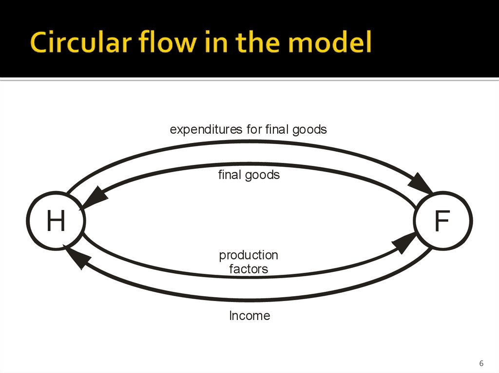
6. Circular flow in the model

expenditures for final goods
final goods
H
F
production
factors
Income
6

7. The essence of aggregate demand

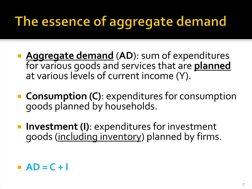
Aggregate demand (AD): sum of expenditures
for various goods and services that are planned
at various levels of current income (Y).
Consumption (C): expenditures for consumption
goods planned by households.
Investment (I): expenditures for investment
goods (including inventory) planned by firms.
AD = C + I
7

8. Consumption component of AD

Two things concerning „C” must be noted:
it is directly dependent on households’ income
it can be financed not only by current income but also
by past or future income
The relationship between „C” and current
income can be presented as marginal
propensity to consume (MPC).
The part of „C” which is independent of current
income is known as autonomous consumption
(CA).
8

9. Marginal propensity to consume

(MPC):
the fraction of the additional current income
which households are going to spend on
additional consumption.
MPC = ΔC/ΔY
9

10. Autonomous consumption

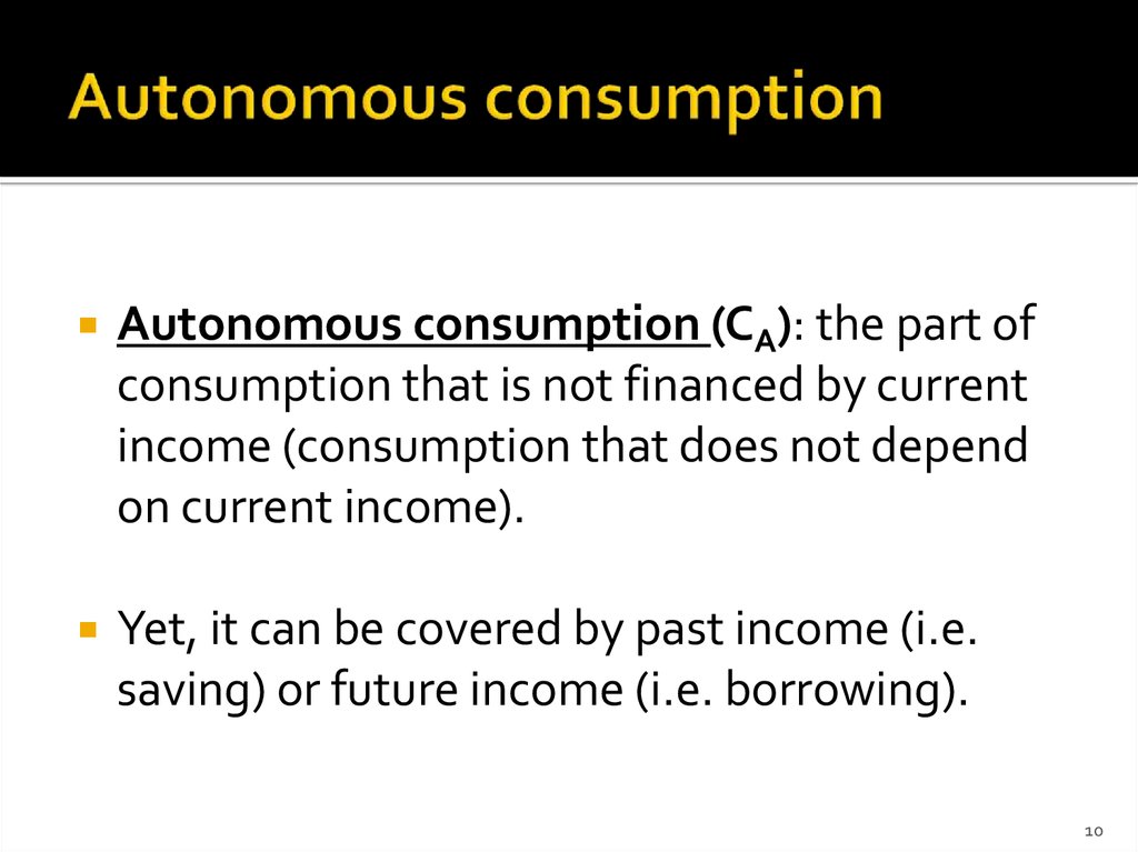
(CA): the part of
consumption that is not financed by current
income (consumption that does not depend
on current income).
Yet, it can be covered by past income (i.e.
saving) or future income (i.e. borrowing).
10

11. Consumption function

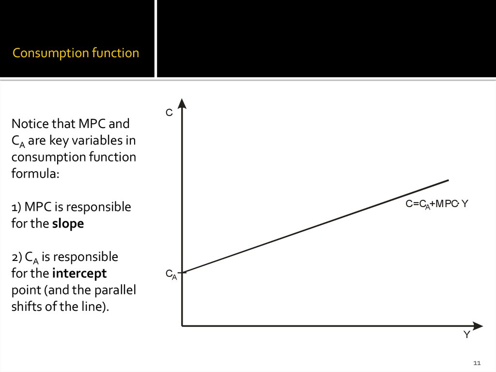
Notice that MPC and
CA are key variables in
consumption function
formula:
C
C=CA+MPC. Y
1) MPC is responsible
for the slope
2) CA is responsible
for the intercept
point (and the parallel
shifts of the line).
CA
Y
11

12. Technical note

Changes in nouseholds’ current income result
in shifts along the consumpion line.
Changes in the autonomous consumption
result in parallel movements of the
consumption line.
Changes in MPC result in the different angle
of the consumption line.
12

13. Saving

means unconsumed income.
Y=C+S
C = MPC×Y + CA
S = MPS×Y – CA
Marginal propensity to save (MPS):
the fraction of the additional current income
which households are going to save.
13

14. Saving function

Notice that saving
function is the mirror
reflection of the
consumption function
formula:
S
S= - CA+MPS.Y
1) MPS is responsible
for the slope
Y
2) CA is responsible
for the intercept
point.
- CA
14

15. Investment component of AD

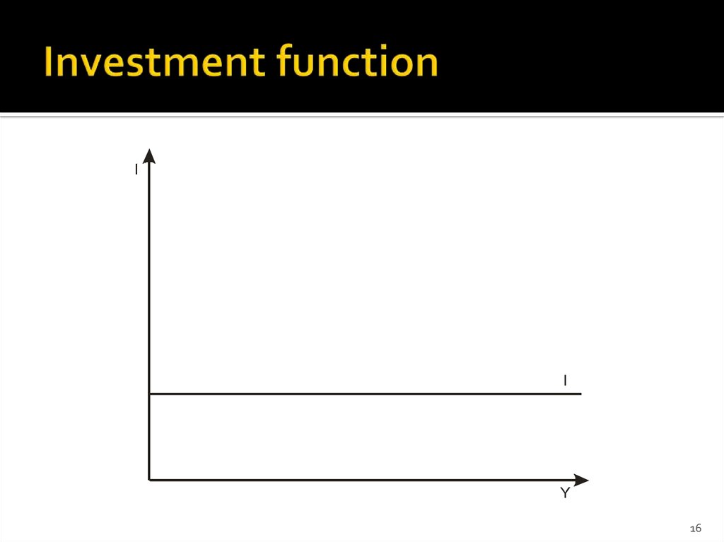
Special status in the Keynesian doctrine
Outstanding variability
Independent of the current state of the economy
(including current income); in that sense they’re
fully autonomous
Dependent on factors such as:
expectations concerning future terms of business
interest rates
15

16. Investment function

I
I
Y
16

17. Aggregate demand: recollection

Aggregate demand: the sum of households’
and firms’ expenditures (for consumption and
investments, respectively) planned at various
levels of current income.
AD = C + I
17

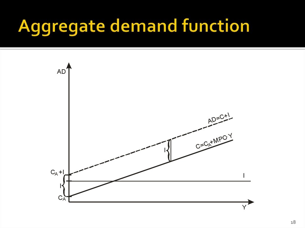
18. Aggregate demand function

AD
C+I
=
D
A
.Y
I
CA +I
MPC
+
C
A
C=
I
I
CA
Y
18

19. 45 degrees line

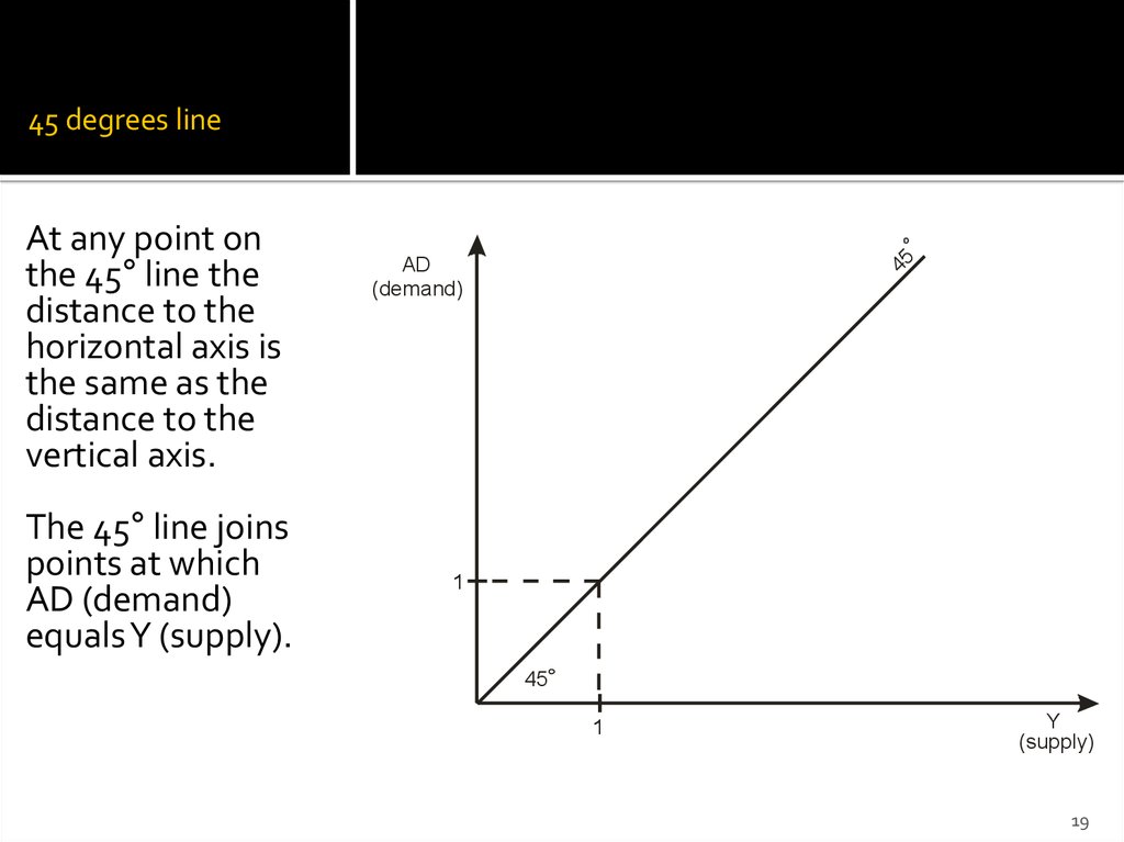
The 45° line joins
points at which
AD (demand)
equalsY (supply).
AD
(demand)
45
At any point on
the 45° line the
distance to the
horizontal axis is
the same as the
distance to the
vertical axis.
1
45
1
Y
(supply)
19

20. Check point: the meaning of „Y”

So far the letter „Y” was using to denote
„income”.
From now on it will be used to denote not
only „income” but also „production”.
How can we justify such decision?
20

21. Keynesian cross

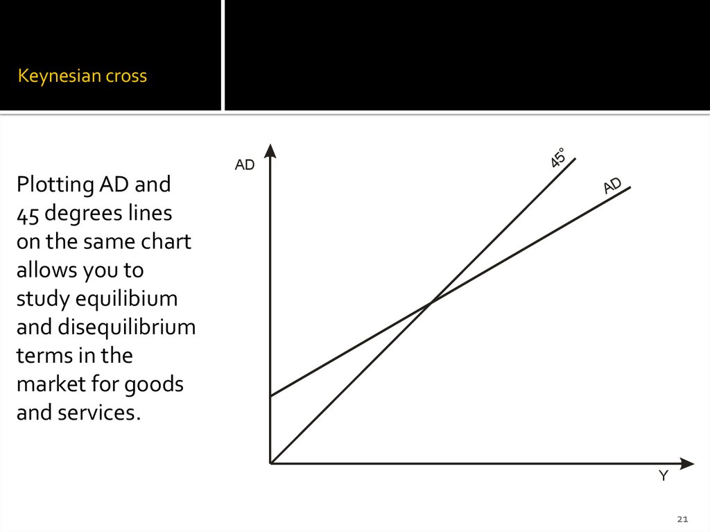
AD
Plotting AD and
45 degrees lines
on the same chart
allows you to
study equilibium
and disequilibrium
terms in the
market for goods
and services.
45
Keynesian cross
AD
Y
21

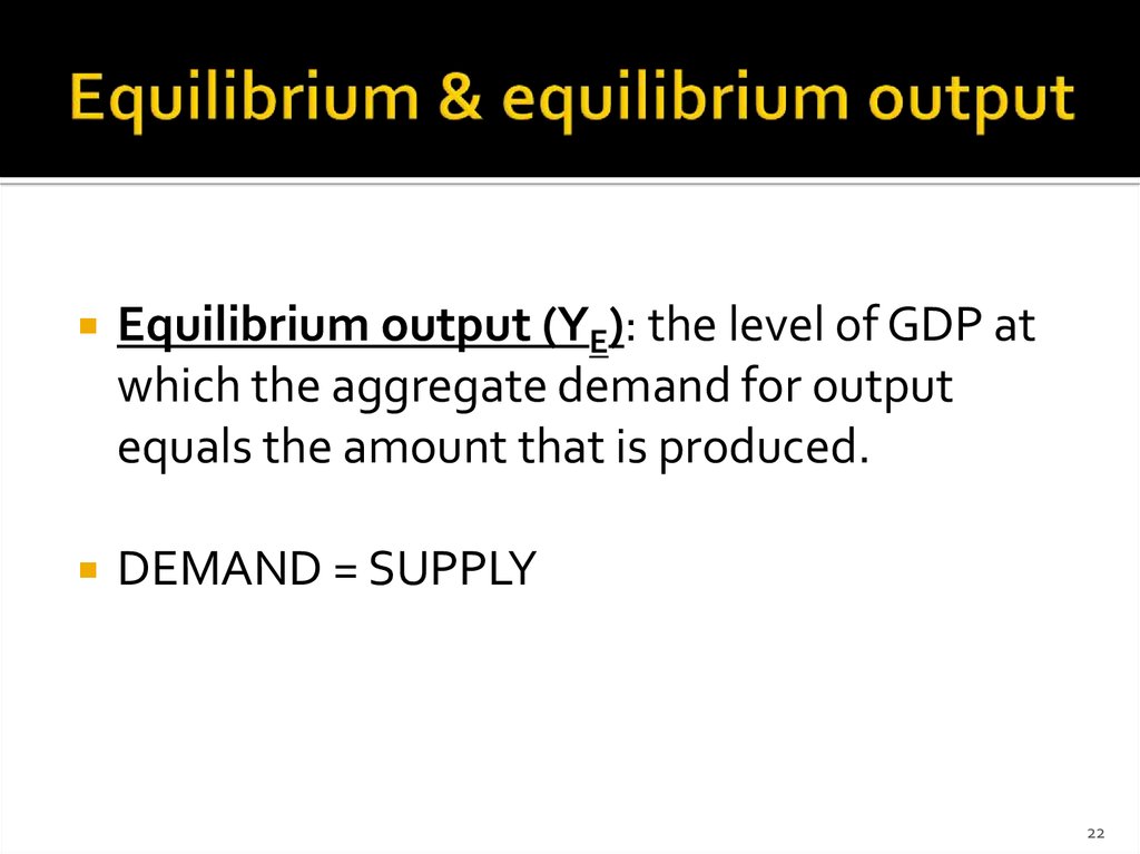
22. Equilibrium & equilibrium output

Equilibrium output (YE): the level of GDP at
which the aggregate demand for output
equals the amount that is produced.
DEMAND = SUPPLY
22

23. Short-run equilibrium in the market for goods and services

45
AD
AD>Y
AD E
AD<Y
=
AD
I
C+
C
.
E
CA
YE
Y
S
S, I
I
-CA
YE
Y
23

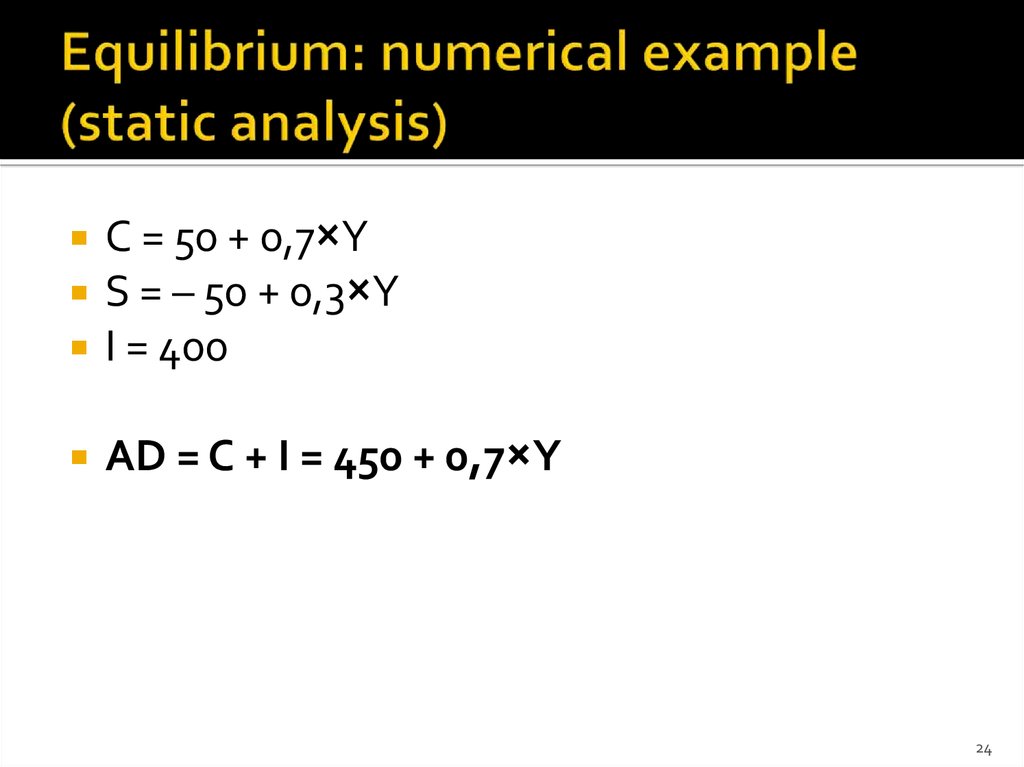
24. Equilibrium: numerical example (static analysis)

C = 50 + 0,7×Y
S = – 50 + 0,3×Y
I = 400
AD = C + I = 450 + 0,7×Y
24

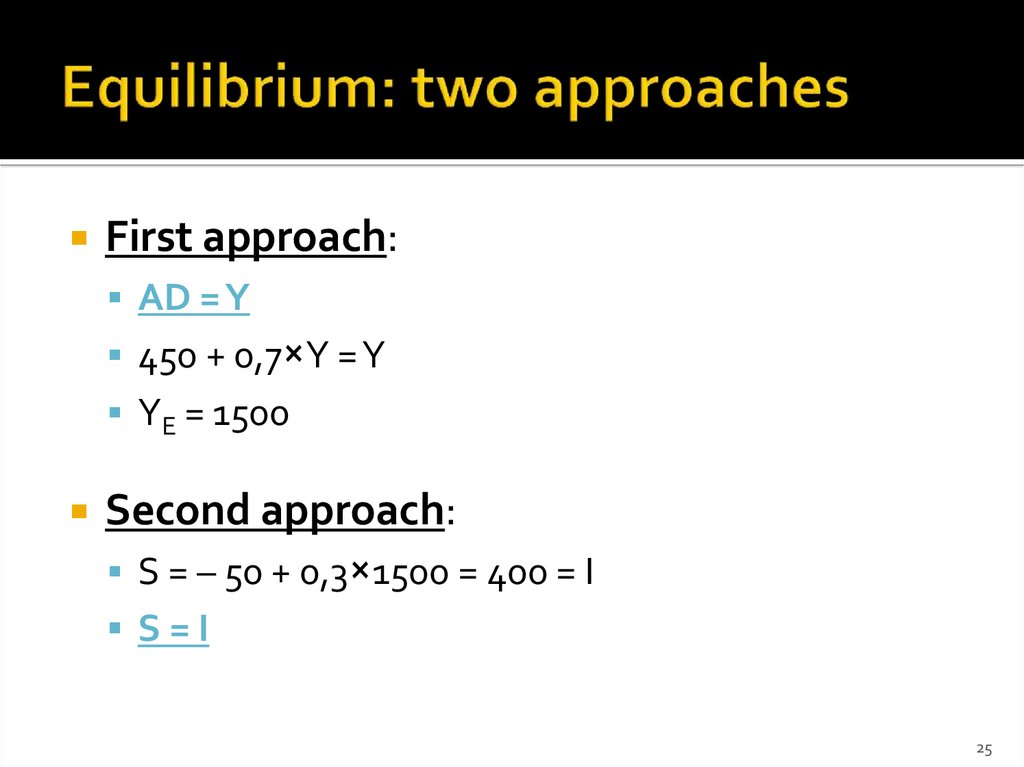
25. Equilibrium: two approaches

First approach:
AD = Y
450 + 0,7×Y = Y
YE = 1500
Second approach:
S = – 50 + 0,3×1500 = 400 = I
S=I
25

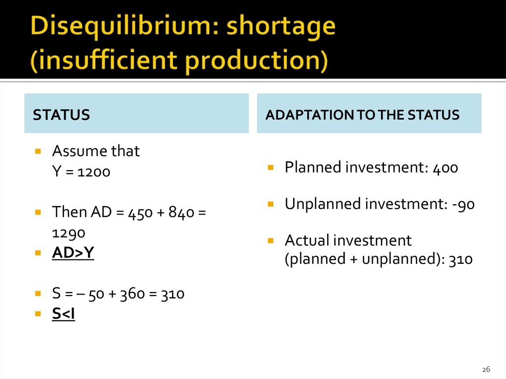
26. Disequilibrium: shortage (insufficient production)

STATUS
Assume that
Y = 1200
Then AD = 450 + 840 =
1290
AD>Y
S = – 50 + 360 = 310
S<I
ADAPTATION TO THE STATUS
Planned investment: 400
Unplanned investment: -90
Actual investment
(planned + unplanned): 310
26

27. Disequilibrium: surplus (excess production)

STATUS
Assume that
Y = 1800
Then AD = 450 + 1260 =
1710
AD<Y
S = – 50 + 540 = 490
S>I
ADAPTATION TO THE STATUS
Planned investment: 400
Unplanned investment: 90
Actual investment
(planned + unplanned): 490
27

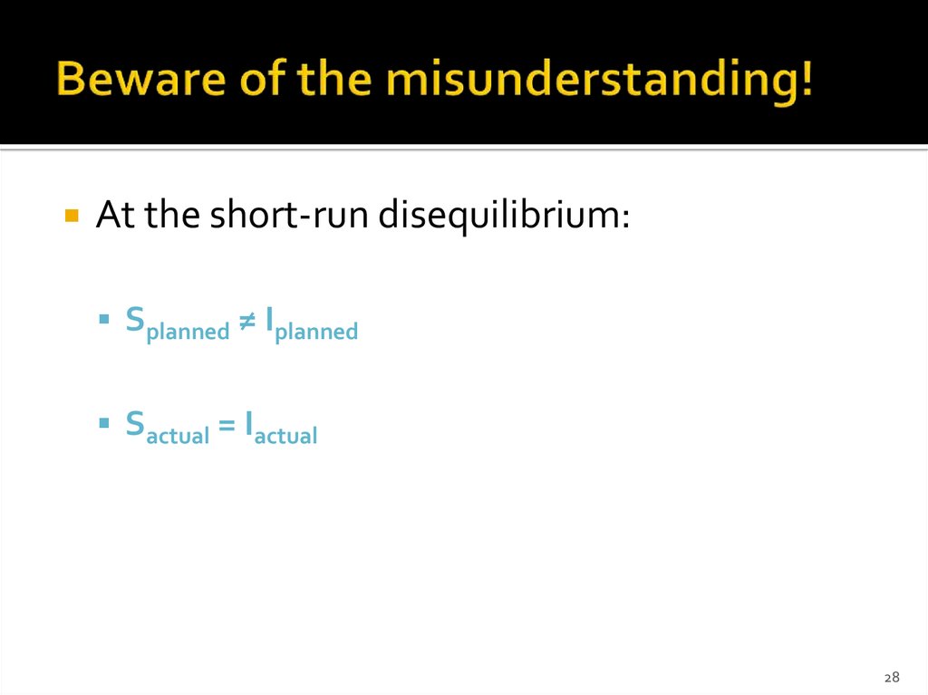
28. Beware of the misunderstanding!

At the short-run disequilibrium:
Splanned ≠ Iplanned
Sactual = Iactual
28

29. Equilibrium: numerical example (dynamic analysis)

Assume that:
C = 50 + 0,7×Y
I = 400 → I’ = 550 (ΔI = 150)
AD’ = 600 + 0,7×Y
YE’ = 2000
YE’ = 2.000
ΔYE/ΔI = 500/150 = 3,33
29

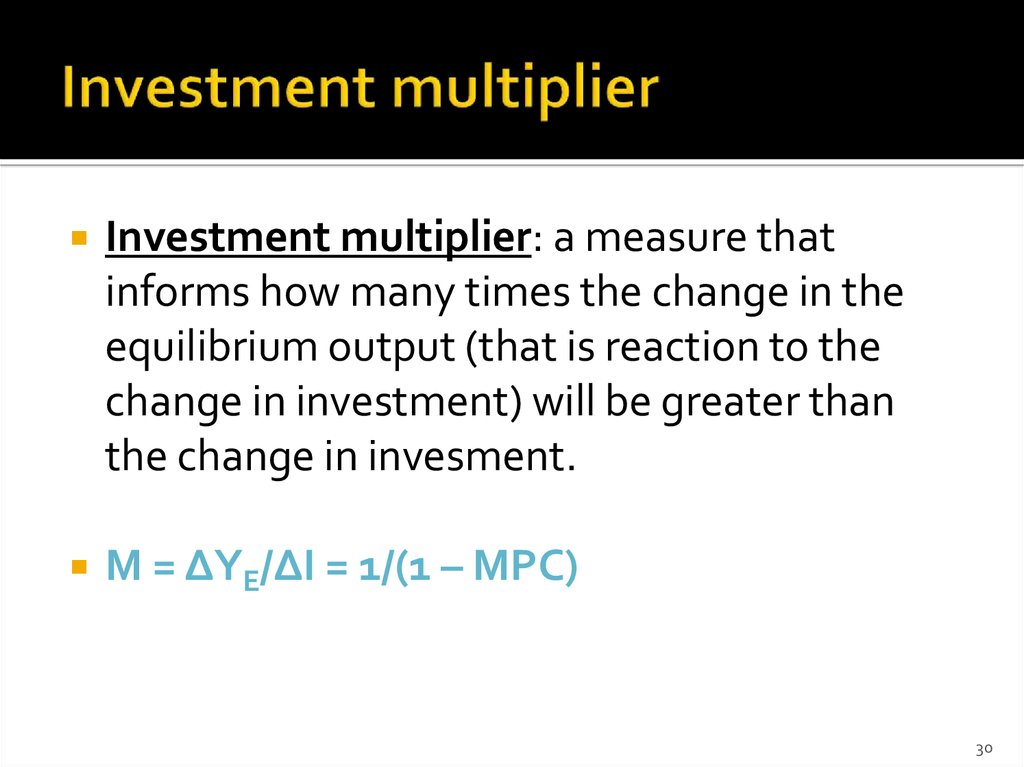
30. Investment multiplier

Investment multiplier: a measure that
informs how many times the change in the
equilibrium output (that is reaction to the
change in investment) will be greater than
the change in invesment.
M = ΔYE/ΔI = 1/(1 – MPC)
30

31. Investment multiplier and economic cycles

Higher multiplier >>> more volatile GDP
Lower multiplier >>> less volatile GDP
31

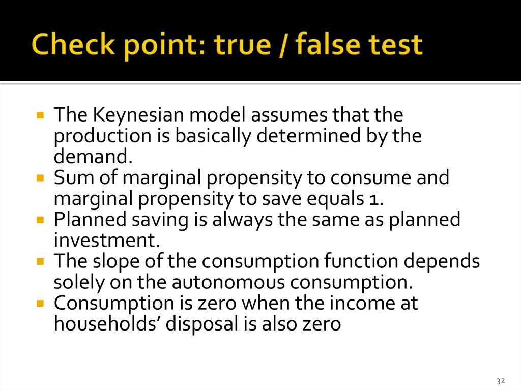
32. Check point: true / false test

The Keynesian model assumes that the
production is basically determined by the
demand.
Sum of marginal propensity to consume and
marginal propensity to save equals 1.
Planned saving is always the same as planned
investment.
The slope of the consumption function depends
solely on the autonomous consumption.
Consumption is zero when the income at
households’ disposal is also zero
32

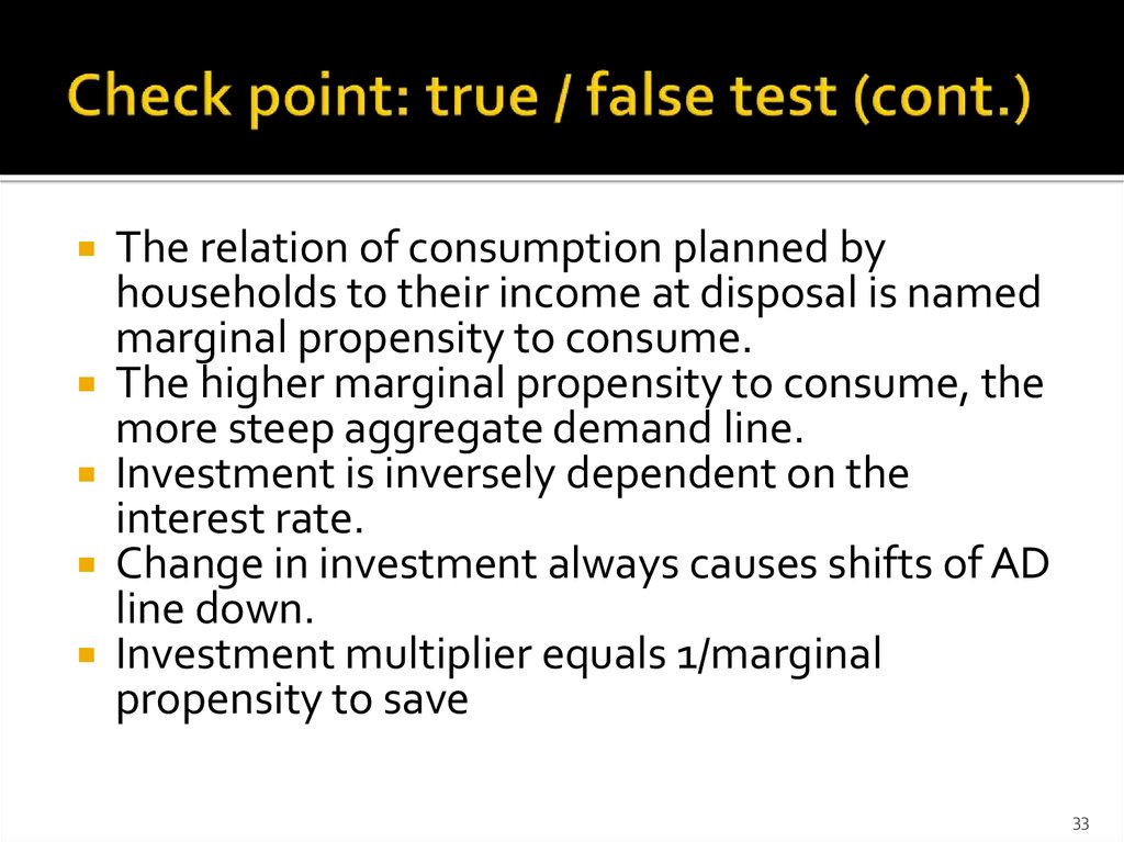
33. Check point: true / false test (cont.)

The relation of consumption planned by
households to their income at disposal is named
marginal propensity to consume.
The higher marginal propensity to consume, the
more steep aggregate demand line.
Investment is inversely dependent on the
interest rate.
Change in investment always causes shifts of AD
line down.
Investment multiplier equals 1/marginal
propensity to save
33

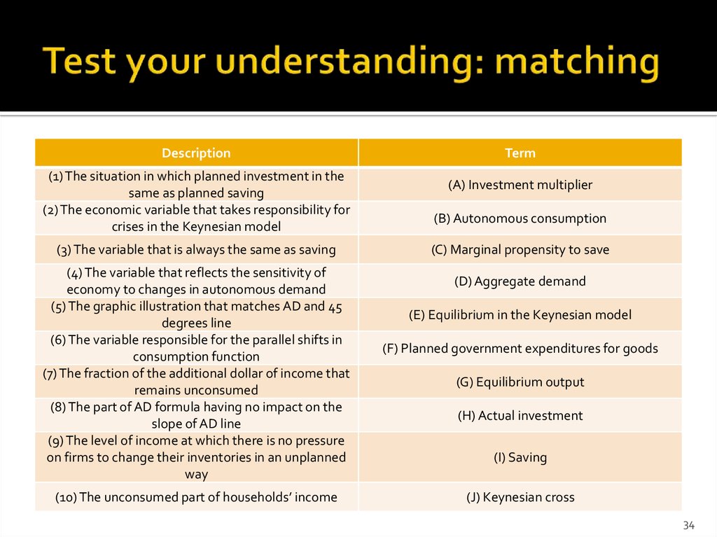
34. Test your understanding: matching

Description
(1) The situation in which planned investment in the
same as planned saving
(2) The economic variable that takes responsibility for
crises in the Keynesian model
(3) The variable that is always the same as saving
(4) The variable that reflects the sensitivity of
economy to changes in autonomous demand
(5) The graphic illustration that matches AD and 45
degrees line
(6) The variable responsible for the parallel shifts in
consumption function
(7) The fraction of the additional dollar of income that
remains unconsumed
(8) The part of AD formula having no impact on the
slope of AD line
(9) The level of income at which there is no pressure
on firms to change their inventories in an unplanned
way
(10) The unconsumed part of households’ income
Term
(A) Investment multiplier
(B) Autonomous consumption
(C) Marginal propensity to save
(D) Aggregate demand
(E) Equilibrium in the Keynesian model
(F) Planned government expenditures for goods
(G) Equilibrium output
(H) Actual investment
(I) Saving
(J) Keynesian cross
34

35. Lecture objectives

What is the essence of the Keynesian
doctrine?
How can economic crises be explained by the
aggregate demand declines?
What are the key factors determining
consumption and investment?
What is the meaning of so called „multiplier”
in the vulnerability of the economy to crises?
35

36. Textbooks

O’Sullivan & Sheffrin: chapter 11, „The
Income-Expenditure Model”
Krugman & Wells: chapter 27, „Dochody
i wydatki”
36