Похожие презентации:
Social Simulation – an introduction
1. Social Simulation – an introduction
Bruce EdmondsCentre for Policy Modelling
Manchester Metropolitan University
2. About Modelling
3. What is a model?
Something, A, that is used to understand or
answer questions about something else, B
e.g: A scale model to test in a wind tunnel
e.g: The official accounts of a business
e.g: The minutes of a meeting
e.g: A flow chart of a legal process
e.g: A memory of a past event
e.g: A computer simulation of the weather
e.g: The analogy of fashion as a virus
Models usually abstract certain features and have
other features that are irrelevant to what is modelled
An Introduction to SS. By Bruce Edmonds, ISS Course, 2011, slide 3
4. A simple consequence of this…
• That if you are only exploring a model to findout about the model, then this is useless,
unless…:
• This understanding helps one understand
other models, for example:
– An idea about something – this is generally private
but not publically useful knowledge
– Or is of SUCH generality it informs us about SO
many other models that it is worth adsorbing
• Normally we use a model to tell us about
something else, something observed (maybe
via intermediate models, such as data)
An Introduction to SS. By Bruce Edmonds, ISS Course, 2011, slide 4
5. What is a formal model?
Something that (in theory) can be writtendown precisely, whose content is
specified without ambiguity
• e.g: mathematical/statistical relations,
computer programs, sets of legal rules
Can make exact copies of it
Agreed rules for interpreting/using them
Can make certain inferences from them
• Not: an analogy, a memory, a physical thing
An Introduction to SS. By Bruce Edmonds, ISS Course, 2011, slide 5
6. The Model and its Target
Object SystemThe mapping
between formal
model and what the
parts refer to
Model
• A formal model is not a model at all without
this mapping relation telling us the intended
meaning of its parts
An Introduction to SS. By Bruce Edmonds, ISS Course, 2011, slide 6
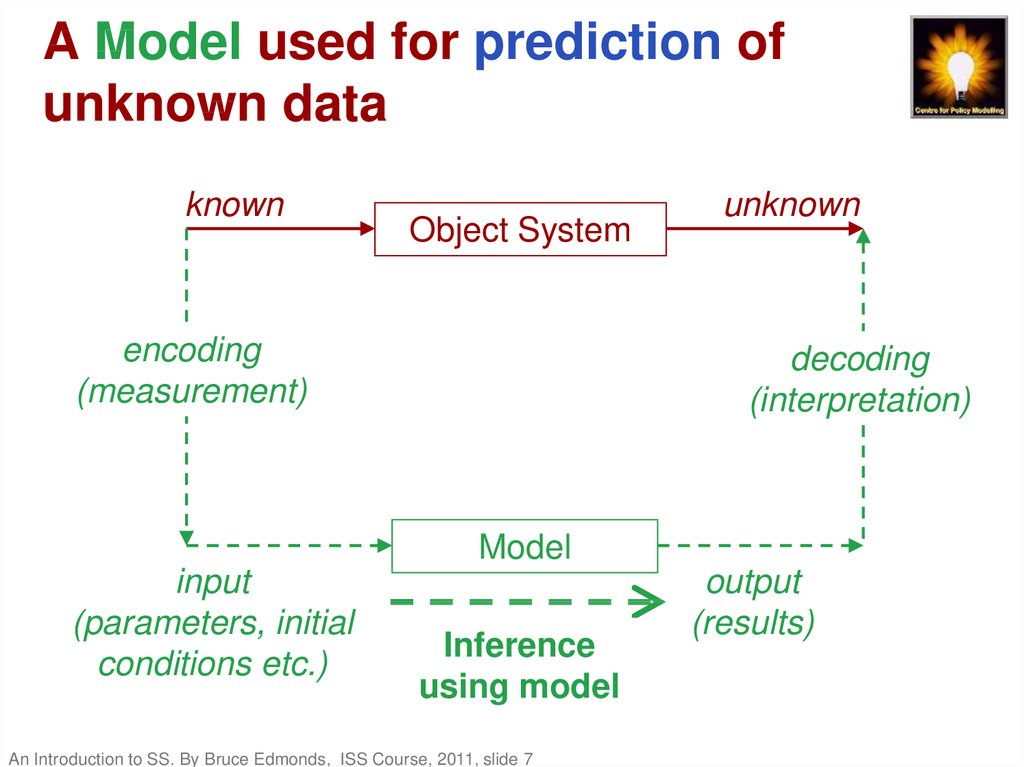
7. A Model used for prediction of unknown data
knownObject System
encoding
(measurement)
unknown
decoding
(interpretation)
Model
input
(parameters, initial
conditions etc.)
Inference
using model
An Introduction to SS. By Bruce Edmonds, ISS Course, 2011, slide 7
output
(results)
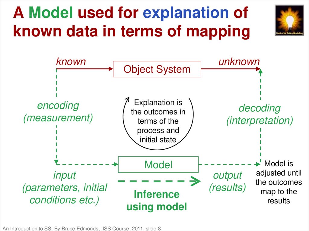
8. A Model used for explanation of known data in terms of mapping
knownencoding
(measurement)
Object System
Explanation is
the outcomes in
terms of the
process and
initial state
unknown
decoding
(interpretation)
Model
input
(parameters, initial
conditions etc.)
Inference
using model
An Introduction to SS. By Bruce Edmonds, ISS Course, 2011, slide 8
output
(results)
Model is
adjusted until
the outcomes
map to the
results
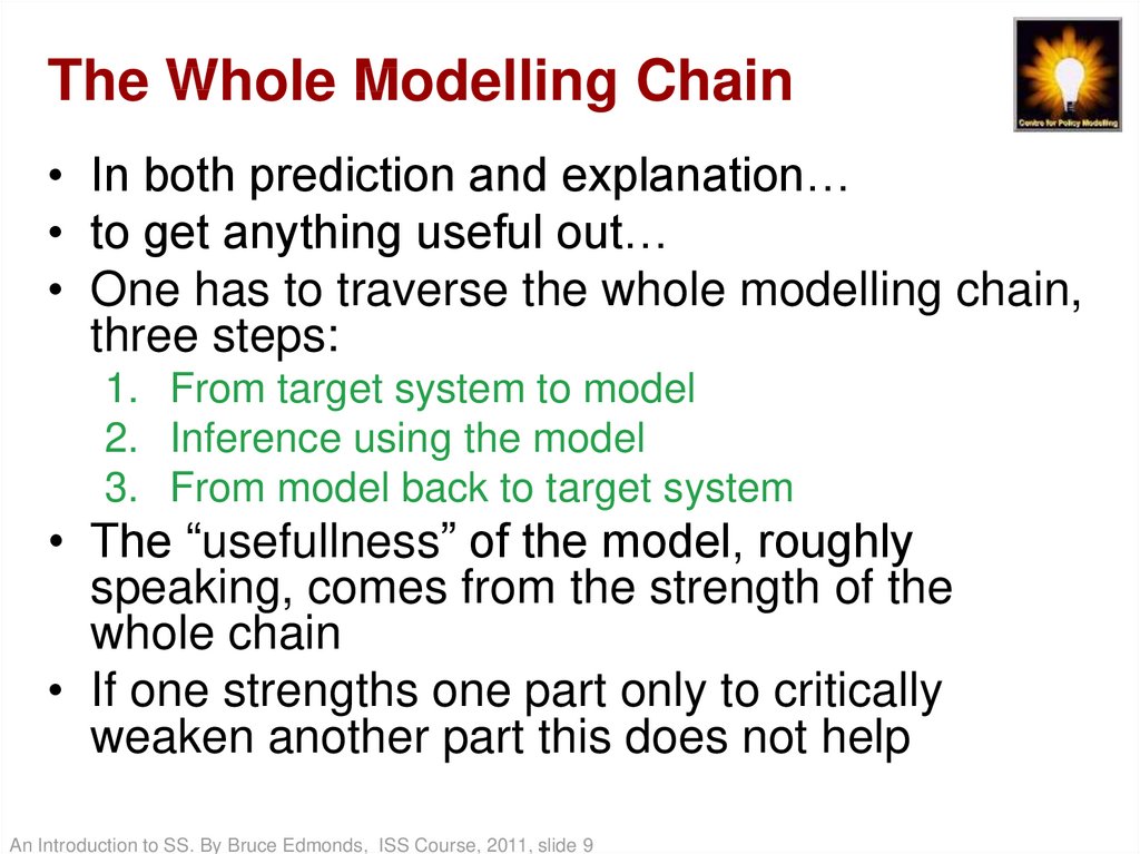
9. The Whole Modelling Chain
• In both prediction and explanation…• to get anything useful out…
• One has to traverse the whole modelling chain,
three steps:
1. From target system to model
2. Inference using the model
3. From model back to target system
• The “usefullness” of the model, roughly
speaking, comes from the strength of the
whole chain
• If one strengths one part only to critically
weaken another part this does not help
An Introduction to SS. By Bruce Edmonds, ISS Course, 2011, slide 9
10. Modelling Purposes
All modelling has a purpose (or several)Including:
• Description
• Prediction
• Establishing/suggesting explanations
• Illustration/communication
• Exploration
• Analogy
These are frequently conflated!
An Introduction to SS. By Bruce Edmonds, ISS Course, 2011, slide 10
11. The Modelling Context
All modelling has a context
The background or situation in which the
modelling occurs and should be interpreted
Whether explicit or (more normally) implicit
Usually can be identified reliably but not
described precisely and completely
The context inevitably hides many implicit
assumptions, facts and processes
Modelling only works if there is a reliably
identifiable context to model within
An Introduction to SS. By Bruce Edmonds, ISS Course, 2011, slide 11
12. Analytic formal models
Where the model is expressed in terms thatallow for formal inferences about its
general properties to be made
• e.g. Mathematical formulae
• Where you don’t have to compute the
consequences but can derive them logically
• Usually requires numerical representation of
what is observed (but not always)
Only fairly “simple” mathematical models can be
treated analytically – the rest have to be
simulated/calculated
An Introduction to SS. By Bruce Edmonds, ISS Course, 2011, slide 12
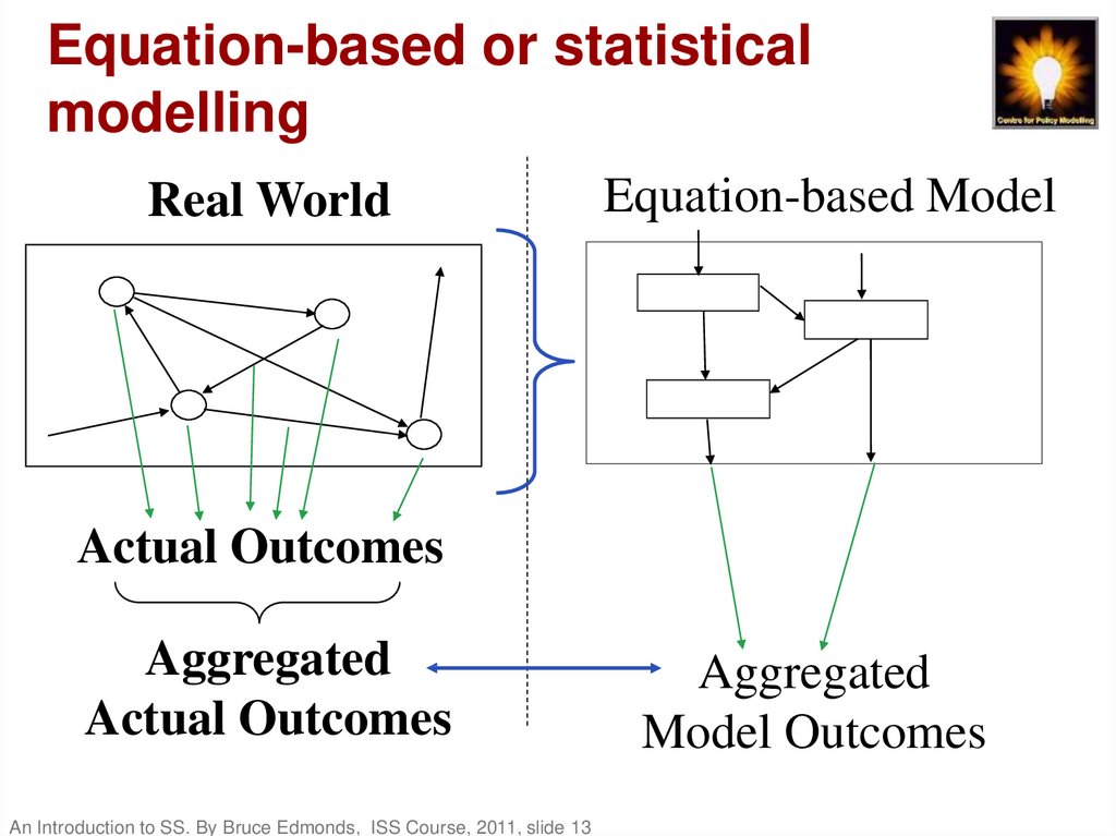
13. Equation-based or statistical modelling
Real WorldEquation-based Model
Actual Outcomes
Aggregated
Actual Outcomes
An Introduction to SS. By Bruce Edmonds, ISS Course, 2011, slide 13
Aggregated
Model Outcomes
14. Computational models
Where a process is modelled in a series of
precise instructions (the program) that can
be “run” on a computer
The same program always produces the same
results (essentially) but...
...may use a “random seed” to randomise
certain aspects
Can be simple or very complex
Often tries to capture more “qualitative”
aspects of phenomena
A computational model of social phenomena is
a social simulation
An Introduction to SS. By Bruce Edmonds, ISS Course, 2011, slide 14
15. Origins of Social Simulation
(Occasionally) Interacting Streams:– Sociology, including social network analysis
– Distributed Computer Science Programming
Languages
– Artificial Intelligence & Machine Learning
– Ecological Modelling
(Strangely) Not much from:
–
–
–
–
(Mainstream) Economics
Cognitive Modelling
Numerical Simulation
System Dynamics
An Introduction to SS. By Bruce Edmonds, ISS Course, 2011, slide 15
16. Two Different Directions
1. Towards the detailed interaction betweenentities
– Trying to capture how the complex interaction
between decision-making actors might result
in the “unexpected” emergence of outcomes
– Roughly this is Agent-based simulation
2. Towards the detail of circumstance
– Trying to use data that allows different regions
or cases to be captured by different models
– Roughly this is Microsimulation
An Introduction to SS. By Bruce Edmonds, ISS Course, 2011, slide 16
17. Other kinds of social simulation model
• Cellular Automaton Models – where patches ina surface change state in response to their
neighbours’ states
• System Dynamic Models – where a system of
equations representing top-level, aggregate
variables are related, then computationally
simulated (sometimes with animation)
• Population Dynamics Models – where a
statistical distribution represents a collection of
individuals plus how these distributions change
over time
An Introduction to SS. By Bruce Edmonds, ISS Course, 2011, slide 17
18. A little bit about Microsimulation
19. About Microsimulation
• Instead of having a generic process over all relevantsituations one has a model for each situation
• This is limited and determined by available data for each
of these situations
• Often these situations are geographical regions
• Often each model is a population dynamics model with
a different distribution for each region, trained on
available data (usually each distribution come from a
family which encode assumptions about the processes)
• Thus variation is not handled by some generic “noise”
but rather aggregation is put off to a post-hoc summary
of the complex results retaining the context-specificity
• This approach is heavily data-driven
• You have to look at each separate region to determine if
the local model is a good fit in each case
An Introduction to SS. By Bruce Edmonds, ISS Course, 2011, slide 19
20. Microsimulation
Observed WorldComputational Model
Outcomes
Model Outcomes
Aggregated
Outcomes
Aggregated
Model Outcomes
An Introduction to SS. By Bruce Edmonds, ISS Course, 2011, slide 20
21. Example 1: General Election Forecasting
• John Curtice(Strathclyde) and
David Firth
(Warwick) (+ input
from others)
• Each constituency
is statistically
modelled as a
three-way split
(Lab, Con, LD)
based on how
much this swung
with the general
trend according to
past data
An Introduction to SS. By Bruce Edmonds, ISS Course, 2011, slide 21
22. Example 1: General Election Forecasting
• Each line is the3-way vote share
for each
constituency in
UK general
elections,
• green spots
show 2005
shares, tail is the
2001 shares
23. Pros and Cons of Microsimulation
Advantages• Data-driven
• Allows for local
differences (contextsensitive)
• Assumptions are
statistical rather
than behavioural
• Relates well to
maps and hence
results are readily
communicable
Disadvantages
• Needs a lot of data at
the granularity being
modelled
• Does not (without
extension) capture
interactions between
regions
• Can take a lot of
computer power
• Does not result in a
simple explanation or
abstraction
An Introduction to SS. By Bruce Edmonds, ISS Course, 2011, slide 23
24. Much more about Agent-Based Social Simulation
25. Some Key Historical Figures
• Herbert Simon– Observed administrative behaviour and described
it using algorithms – ‘procedural rationality’ (rather
than optimisation of utility)
– Also (with Alan Newell) produced first
computational models of aspects of cognition
• Thomas Schelling
– A simple but effective example of individual-based
modelling (in the coming slides) showing power of
simulation establishing a micro-macro link
• Mark Granovetter
– Distinguished the importance of tracing individual
interactions, ‘social embeddedness’
– Highlighted such processes and structure (‘ties’)
An Introduction to SS. By Bruce Edmonds, ISS Course, 2011, slide 25
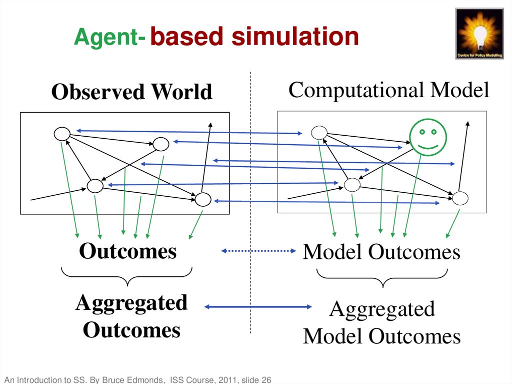
26. Individual-based simulation
AgentIndividual-basedsimulation
Observed World
Computational Model
Outcomes
Model Outcomes
Aggregated
Outcomes
Aggregated
Model Outcomes
An Introduction to SS. By Bruce Edmonds, ISS Course, 2011, slide 26
27. Micro-Macro Relationships
Macro/Social data
Social, economic surveys; Census
Theory,
narrative
accounts
Micro/
Individual data
Simulation
Qualitative, behavioural, social psychological data
An Introduction to SS. By Bruce Edmonds, ISS Course, 2011, slide 27
28. Characteristics of agent-based modelling
Computational description of process
Not usually analytically tractable
More context-dependent…
… but assumptions are much less drastic
Detail of unfolding processes accessible
– more criticisable (including by non-experts)
• Used to explore inherent possibilities
• Validatable by data, opinion, narrative ...
• Often very complex themselves
An Introduction to SS. By Bruce Edmonds, ISS Course, 2011, slide 28
29. What happens in ABSS
• Entities in simulation are decided up• Behavioural Rules for each agent specified (e.g. sets of
rules like: if this has happened then do this)
• Repeatedly evaluated in parallel to see what happens
• Outcomes are inspected, graphed, pictured, measured
and interpreted in different ways
Specification (incl. rules)
Representations of Outcomes
Simulation
An Introduction to SS. By Bruce Edmonds, ISS Course, 2011, slide 29
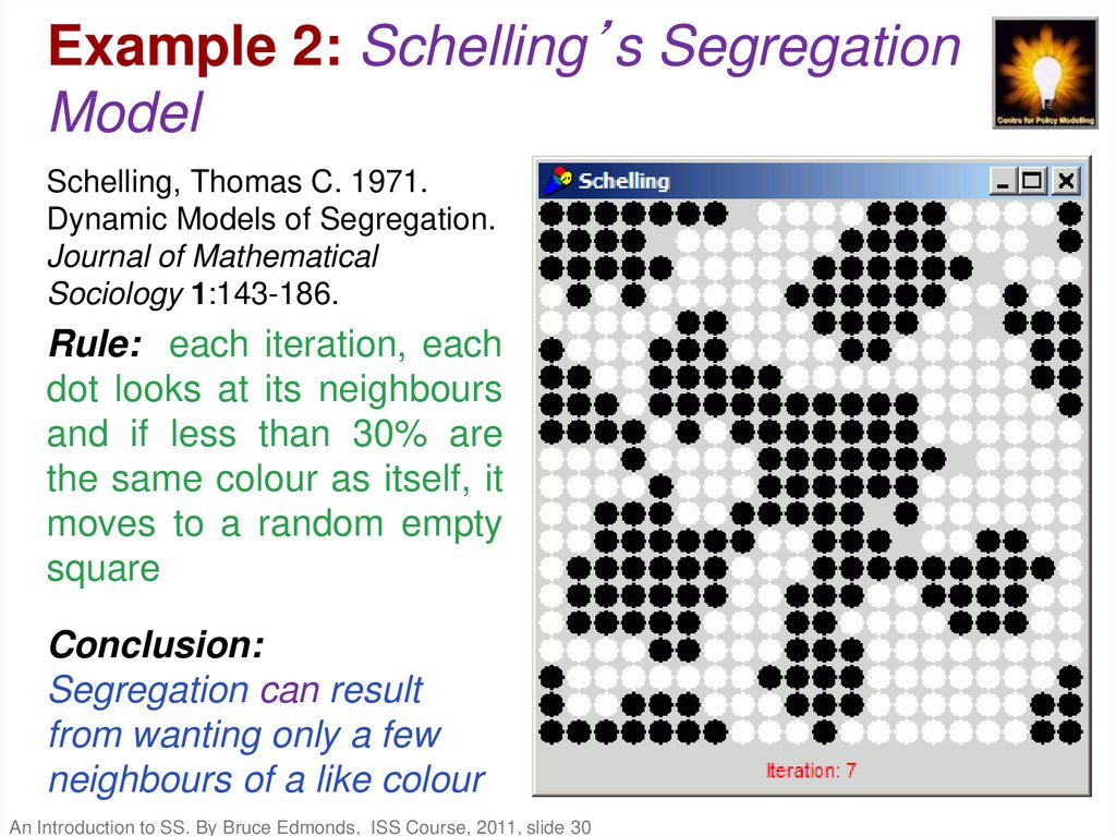
30. Example 2: Schelling’s Segregation Model
Schelling, Thomas C. 1971.Dynamic Models of Segregation.
Journal of Mathematical
Sociology 1:143-186.
Rule: each iteration, each
dot looks at its neighbours
and if less than 30% are
the same colour as itself, it
moves to a random empty
square
Conclusion:
Segregation can result
from wanting only a few
neighbours of a like colour
An Introduction to SS. By Bruce Edmonds, ISS Course, 2011, slide 30
31. Simple, Conceptual Simulations Such as Schelling’s
• Are highly suggestive• Once you play with them, you start to “see”
the world in terms of you model – a strong
version of Kuhn’s theoretical spectacles
• They can help persuade beyond the limit of
their reliability
• They may well not be directly related to any
observations of social phenomena
• Are more a model of an idea than any
observed phenomena
• Can be used as a counter-example
An Introduction to SS. By Bruce Edmonds, ISS Course, 2011, slide 31
32. Modelling a concept of something
PhenomenaAnalogical
Application
conceptual model
Exploration
with model
Model
An Introduction to SS. By Bruce Edmonds, ISS Course, 2011, slide 32
33. Some Criteria for Judging a Model
• Soundness of design– w.r.t. knowledge of how the object works
– w.r.t. tradition in a field
• Accuracy (lack of error)
• Simplicity (ease in communication,
construction, comprehension etc.)
• Generality (when you can safely use it)
• Sensitivity (relates to goals and object)
• Plausibility (of design, process and results)
• Cost (time, effort, etc.)
An Introduction to SS. By Bruce Edmonds, ISS Course, 2011, slide 33
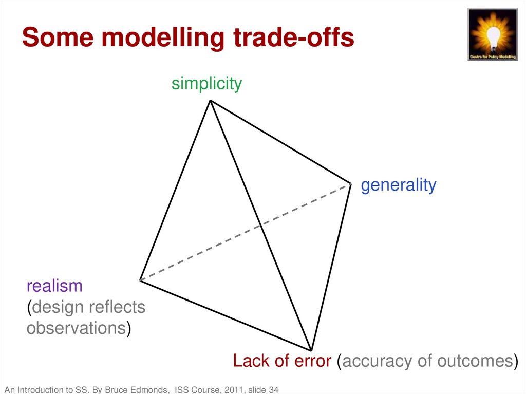
34. Some modelling trade-offs
simplicitygenerality
realism
(design reflects
observations)
Lack of error (accuracy of outcomes)
An Introduction to SS. By Bruce Edmonds, ISS Course, 2011, slide 34
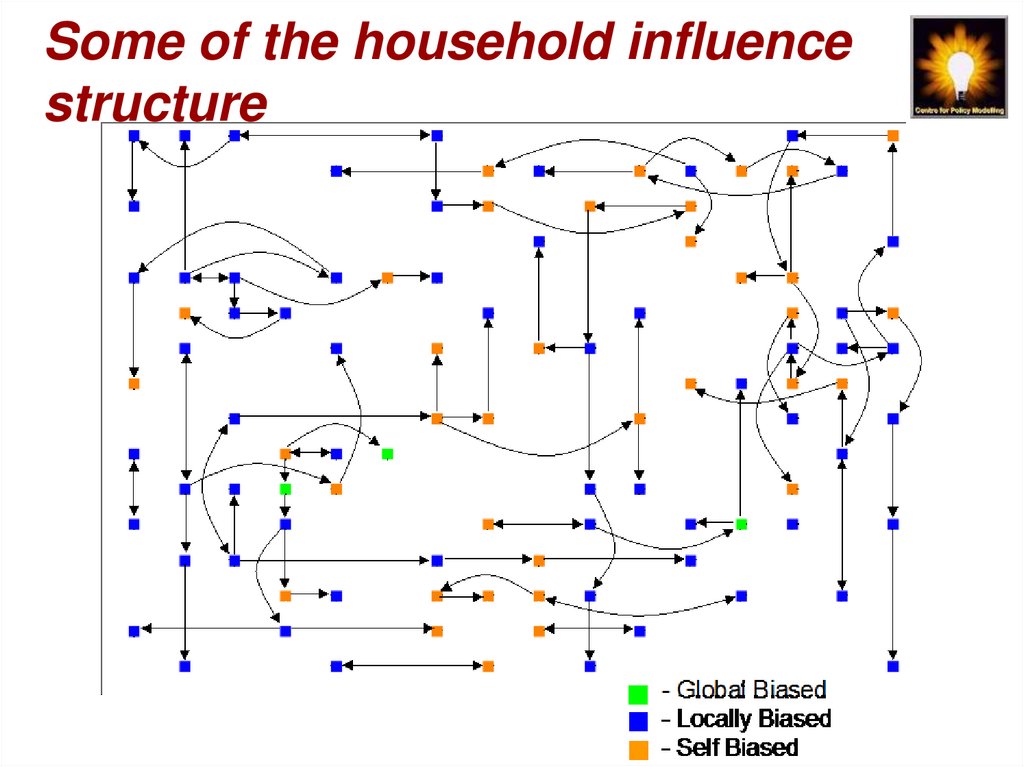
35. Example 3: A model of social influence and water demand
• Investigate the possible impact of socialinfluence between households on patterns
of water consumption
• Design and detailed behavioural outcomes
from simulation validated against expert
and stakeholder opinion at each stage
• Some of the inputs are real data
• Characteristics of resulting aggregate time
series validated against similar real data
An Introduction to SS. By Bruce Edmonds, ISS Course, 2011, slide 35
36. Type, context, purpose
• Type: A complex agent-based descriptivesimulation integrating a variety of streams
of evidence
• Context: statistical and other models of
domestic water demand under different
climate change scenarios
• Purposes:
– to critique the assumptions that may be implicit
in the other models
– to demonstrate an alternative
An Introduction to SS. By Bruce Edmonds, ISS Course, 2011, slide 36
37. Simulation structure
PolicyAgent
•Activity
•Frequency
•Volume
Households
Ground
Aggregate Demand
•Temperature
•Rainfall
•Daylight
An Introduction to SS. By Bruce Edmonds, ISS Course, 2011, slide 37
38. Some of the household influence structure
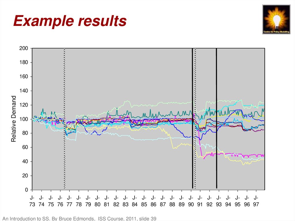
39. Example results
Aggregate demand series scaled so 1973=100200
180
160
Relative Demand
140
120
100
80
60
40
20
0
J- J- J- J- J- J- J- J- J- J- J- J- J- J- J- J- J- J- J- J- J- J- J- J- J73 74 75 76 77 78 79 80 81 82 83 84 85 86 87 88 89 90 91 92 93 94 95 96 97
Simulation Date
An Introduction to SS. By Bruce Edmonds, ISS Course, 2011, slide 39
40. Conclusions from Water Demand Example
• The use of a concrete descriptive simulationmodel allowed the detailed criticism and,
hence, improvement of the model
• The inclusion of social influence resulted in
aggregate water demand patterns with
many of the characteristics of observed
demand patterns
• The model established how it was possible
that processes of mutual social influence
could result in widely differing patterns of
consumption that were self-reinforcing
An Introduction to SS. By Bruce Edmonds, ISS Course, 2011, slide 40
41. What ABSS Can Do
• ABSS can allow the production and examination ofsets of possible complicated processes both
emergent and immergent
• Using a precise (well-defined and replicable)
language (a computer program)
• But one which allows the tracing of very
complicated interactions
• And thus does not need the strong assumptions that
analytic approaches require to obtain their proofs
• It allows the indefinite experimentation and
examination of outcomes (in vitro)
• Which can inform our understanding of some of the
complex interactions that may be involved in
observed (in vivo) social phenomena
An Introduction to SS. By Bruce Edmonds, ISS Course, 2011, slide 41
42. Conclusion
43. The in vitro and in vivo analogy
• In vivo is what happens in real life, e.g.between complex chemicals in the cell
– Any data or experiments here involve the whole
complex context of the target system
– But these are often so complex its impossible to
detangle the interactions at this level
• In vitro is what happens in the test tube with
selected chemicals, it is a model of of the cell
– This allows experiments and probes to tease out
how some of the complex interactions occur
– But you never know if back in the cell these may be
overwhelmed or subverted by other interactions
An Introduction to SS. By Bruce Edmonds, ISS Course, 2011, slide 43
44. Discursive vs Simulation Approaches
Natural LanguageComputer Simulation
• Rich, semantic,
meaningful, flexible
• But imprecise
• Map to what is observed
is often complex and
implicit
• Difficult to keep track of
complicated interactions
and outcomes
• Has “pre-prepared”
meaning and referents
• Precise, well defined,
replicable, flexible
• But brittle
• Semantically thin
• Map to observed can be
explicit and more direct
• Good at keeping track of
complicated interactions
and outcomes
• Meaning needs to be
established through use
An Introduction to SS. By Bruce Edmonds, ISS Course, 2011, slide 44
45. Analytic vs Simulation Approaches
Analytic ModellingComputer Simulation
• Precise, well defined,
replicable
• Very brittle
• Not Semantic
• Map to observed can be
indirect and/or difficult to
establish
• Strong checkable inference
• General characterisation of
outcomes
• Requires strong
assumptions to work
• Precise, well defined,
replicable, flexible
• More expressive
descriptive
• Semantically thin
• Map to observed can be
explicit and more direct
• Inference is more
contingent, (sets of)
example outcomes
• Can relate more easily to a
broader range of evidence
An Introduction to SS. By Bruce Edmonds, ISS Course, 2011, slide 45
46. The End
These slides are accessible from the ‘slides’ link on theIntroduction to Social Simulation Course Page
http://sites.google.com/site/socialsimulationcourse
Bruce Edmonds
http://bruce.edmonds.name
Centre for Policy Modelling
http://cfpm.org
Manchester Metropolitan Business School
http://www.business.mmu.ac.uk
NeISS Portal
http://www.neiss.org.uk

















 Английский язык


