Simple Regression

1.

Regression and Correlation

2. Recall: Covariance

n
cov ( x , y )
X
2
4
3
8
….
Y
5
7
6
5
….
( xi X )( yi Y )
i 1
n 1

3. Interpreting Covariance

cov(X,Y) > 0
X and Y are positively correlated
cov(X,Y) < 0
X and Y are inversely correlated
cov(X,Y) = 0
X and Y are independent

4. Correlation coefficient

Pearson’s Correlation Coefficient is
standardized covariance (unitless):
cov ariance ( x, y)
r
var x var y

5. Correlation

• Measures the relative strength of the linear
relationship between two variables
• Unit-less
• Ranges between –1 and 1
• The closer to –1, the stronger the negative linear relationship
• The closer to 1, the stronger the positive linear relationship
• The closer to 0, the weaker any positive linear relationship

6. Scatter Plots of Data with Various Correlation Coefficients

Y
Y
Y
X
X
r = -1
r = -0.6
Y
r=0
Y
Y
r = +1
X
X
X
r = +0.3
X
r=0

7. Linear Correlation

Linear relationships
Curvilinear relationships
Y
Y
X
Y
X
Y
X
X

8. Linear Correlation

Strong relationships
Weak relationships
Y
Y
X
Y
X
Y
X
X

9. Linear Correlation

No relationship
Y
X
Y
X

10. Calculating by hand…

n
( x x )( y y )
i 1
cov ariance ( x, y )
rˆ
var x var y
n
i
i
n 1
n
2
(
x
x
)
i
2
(
y
y
)
i
n 1
n 1
i 1
i 1

11. Simpler calculation formula…

Numerator of
covariance
n
( x x )( y y )
i
i 1
rˆ
i
n 1
n
n
(x x) ( y y)
2
i 1
i
i 1
n 1
2
i
n 1
rˆ
SS xy
SS x SS y
n
( x x )( y y )
i 1
i
i
n
(x x ) ( y y)
2
i 1
n
i
i 1
i
2
SS xy
SS x SS y
Numerators of
variance

12. Correlation

13. Regression: Introduction

Basic idea:
Use data to identify relationships
among variables and use these
relationships to make predictions.

14. Linear regression

•Linear dependence: constant rate of increase of one variable
with respect to another (as opposed to, e.g., diminishing
returns).
•Regression analysis describes the relationship between two
(or more) variables.
•Examples:
– Income and educational level
– Demand for electricity and the weather
– Home sales and interest rates
•Our focus:
–Gain some understanding of
• the regression line
• regression error
– Learn how to interpret and use the results.
– Learn how to setup a regression analysis.

15. Two main questions:

•Prediction and Forecasting
– Predict home sales for December given the interest rate for this month.
– Use time series data (e.g., sales vs. year) to forecast future performance
(next year sales).
– Predict the selling price of houses in some area.
• Collect data on several houses (# of BR, #R, sq.ft, lot size, property tax) and
their selling price.
• Can we use this data to predict the selling price of a specific house?
•Quantifying causality
– Determine factors that relate to the variable to be predicted; e.g., predict
growth for the economy in the next quarter: use past history on
quarterly growth, index of leading economic indicators, and others.
– Want to determine advertising expenditure and promotion for the 2020.
•Sales over a quarter might be influenced by: ads in print, ads in radio, ads in
TV, and other promotions.

16. Motivated Example

• Predict the selling prices of houses in the region.
• Collect recent historical data on selling prices, and a number of
characteristics about each house sold (size, age, style, etc.).
•One of the factors that cause houses in the data set to sell for
different amounts of money is the fact that houses come in
various sizes.
•A preliminary model might posit that the average value per
square foot of a new house is $40 and that the average lot sells
for $20,000. The predicted selling price of a house of size X (in
square meter) would be: 20,000 + 400X.
•A house of 200 square meter would be estimated to sell for
20,000 + 400(200) = $100,000.

17. Motivated Example

•Probability Model:
– We know, however, that this is just an approximation, and the selling
price of this particular house of 200 square meter is not likely to be
exactly $100,000.
– Prices for houses of this size may actually range from $50,000 to $150,000.
– In other words, the deterministic model is not really suitable. We should
therefore consider a probabilistic model.
•Let Y be the actual selling price of the house. Then
Y = 20,000 + 40x + ,
where (Greek letter epsilon) represents a random error
term (which might be positive or negative).
– If the error term is usually small, then we can say the model is a good
one.
– The random term, in theory, accounts for all the variables that are not
part of the model (for instance, lot size, neighborhood, etc.).
– The value of will vary from sale to sale, even if the house size remains
constant. That is, houses of the exact same size may sell for different
prices.

18. Regression Model

•The variable we are trying to predict (Y) is called the
dependent (or response) variable.
•The variable x is called the independent (or predictor, or
explanatory) variable.
•Our model assumes that
E(Y | X = x) = 0 + 1x
(the “population line”)
(1)
The interpretation is as follows:
–When X (house size) is fixed at a level x, then we assume the mean of Y
(selling price) to be linear around the level x, where 0 is the (unknown)
intercept and 1 is the (unknown) slope or incremental change in Y per
unit change in X.
– 0 and 1 are not known exactly, but are estimated from sample data.
Their estimates are denoted b0 and b1.
•A simple regression model: Consider a model with only one
independent variable,.
•A multiple regression model: a model with multiple
independent variables.

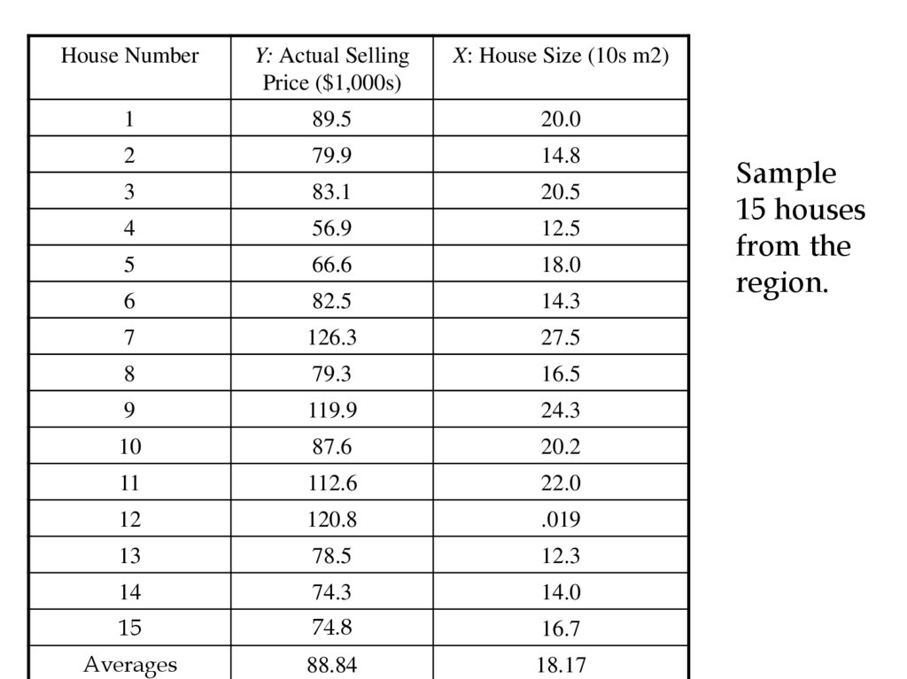
19.

House Number
Y: Actual Selling
Price ($1,000s)
X: House Size (10s m2)
1
89.5
20.0
2
79.9
14.8
3
83.1
20.5
4
56.9
12.5
5
66.6
18.0
6
82.5
14.3
7
126.3
27.5
8
79.3
16.5
9
119.9
24.3
10
87.6
20.2
11
112.6
22.0
12
120.8
.019
13
78.5
12.3
14
74.3
14.0
15
74.8
16.7
Averages
88.84
18.17
Sample
15 houses
from the
region.

20. Least Squares Estimation

•price<- c(89.5,79.9,83.1,56.9,66.6,82.5,126.3,79.3,119.9,87.6,112.6,120.8,78.5,74.3,74.8)
•size<- c(20.0,14.8,20.5,12.5,18.0,14.3,27.5,16.5,24.3,20.2,22.0,19.0,12.3,14.0,16.7)
•plot(size,price,xlab= “House size (100 sq m)”,ylab=“Selling price
($1,000)”,main=“House Size (X) vs Selling Price (Y)”)

21. Assumptions

•These data do not form a perfect line. This is not surprising,
considering that our data are random. In other words, if we
assume equation (1) then our line predicts the mean for any
given level x. However, when we actually take a
measurement (i.e., observe the data), we observe:
Yi = 0 + 1Xi + i,
for i = 1,2,…, n = 15,
where i is the random error associated with the ith
observation.
–Since we don't know the true values of 0 and 1, it is clear that we do
not observe the actual errors ( i) precisely either.
•Assumptions about the Error
–E( i ) = 0 for i = 1, 2,…,n.
– ( i ) = where is unknown.
–The errors are independent, that is, the error in the ith observation is
independent of the error observed in the jth observation.
–The i are normally distributed (with mean 0 and standard deviation ).

22. Least Squares Estimation

•Recall 0 and 1 are (unknown) population parameters.
– From the sample data, we will calculate numbers ˆ0 and ̂1 that are
estimates of the population parameters.
– How should these numbers be chosen? For any choice of ˆ0 and ̂1 ,
we can write the following prediction equation
ŷ = ˆ0 + ̂1 X.
– The “hat” is used to denote a value estimated from the model, as
opposed to one that is actually observed.
– For each house in our sample of 15 we could check to see how well
this equation works at predicting the actual selling prices. Define ei to
be the error associated with the ith observation. That is:
ei = yi - (estimated selling price)
These are sometimes called the residuals or simply errors.
•We will pick the values of ˆ0 and ̂1 that minimize Si ei2, the
sum of the squares of the residuals. This method is often
called Least Squares Regression.

23. Linear Equations

Y
Y = mX + b
m = Slope
Change
in Y
Change in X
b = Y-intercept
X
23

24. Linear Regression Model

• 1. Relationship Between Variables Is a
Linear Function
Population
Y-Intercept
Population
Slope
Random
Error
Yi 0 1X i i
Dependent
(Response)
Variable
(e.g., CD+ c.)
Independent
(Explanatory) Variable
(e.g., Years s. serocon.)

25. Population & Sample Regression Models

Population & Sample Regression
Models
Population
Unknown
Relationship
Yi 0 1X i i
25

26. Population & Sample Regression Models

Population & Sample Regression
Models
Population
Unknown
Relationship
Yi 0 1X i i
Random Sample
Y i 0 1 X i i
26

27. Population Linear Regression Model

Y
Yi 0 1 X i i
Observed
value
i = Random error
E Y 0 1 X i
X
Observed value
27

28. Estimating Parameters: Least Squares Method

28

29. Scatter plot

• 1. Plot of All (Xi, Yi) Pairs
• 2. Suggests How Well Model Will Fit
60
40
20
0
Y
0
20
40
X
60
29

30. Thinking Challenge

How would you draw a line through the
points? How do you determine which line
‘fits best’?
60
40
20
0
Y
0
20
40
X
60
30

31. Least Squares

• 1. ‘Best Fit’ Means Difference Between
Actual Y Values & Predicted Y Values Are
a Minimum. But Positive Differences OffSet Negative ones
31

32. Least Squares

• 1. ‘Best Fit’ Means Difference Between
Actual Y Values & Predicted Y Values Are
a Minimum. But Positive Differences OffSet Negative. So square errors!
n
ˆ
Y
Y
i i
i 1
ˆ
2
n
i 1
2
i
• 2. LS Minimizes the Sum of the Squared
Differences (errors) (SSE)
32

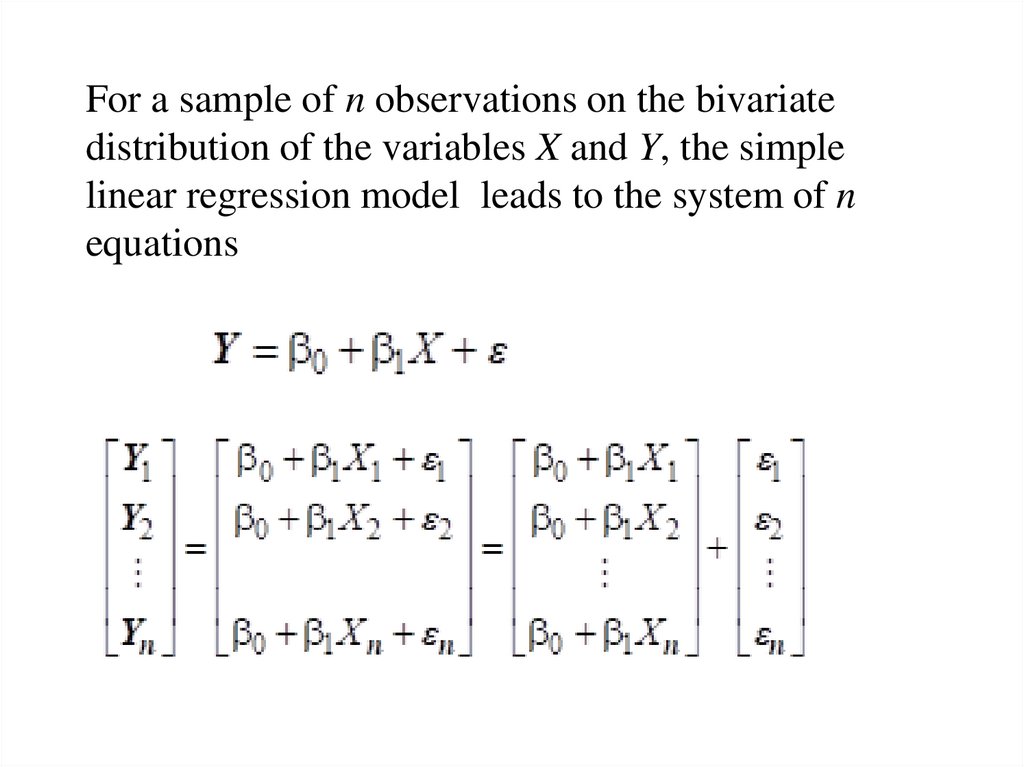
33.

For a sample of n observations on the bivariate
distribution of the variables X and Y, the simple
linear regression model leads to the system of n
equations

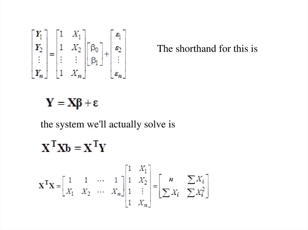
34.

The shorthand for this is
the system we'll actually solve is

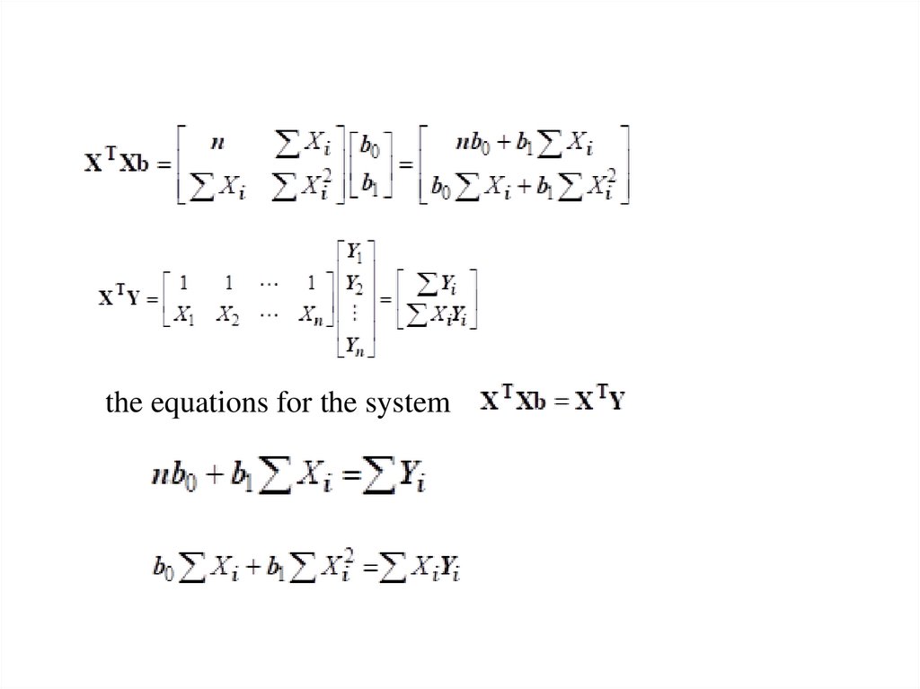
35.

the equations for the system

36. Derivation of Parameters (another way)

• Least Squares (L-S):
Minimize squared error
n
n
yi 0 1 xi
i 1
0
i2
0
2
i
2
i 1
yi 0 1 xi
2
0
2 ny n 0 n 1 x
ˆ0 y ˆ1x
36

37. Derivation of Parameters

• Least Squares (L-S):
Minimize squared error
2
i2
yi 0 1 xi
0
1
1
2 xi yi 0 1 xi
2 xi yi y 1 x 1 xi
1 xi xi x xi yi y
1 xi x xi x xi x yi y
SS xy
ˆ
1
SS xx
37

38.

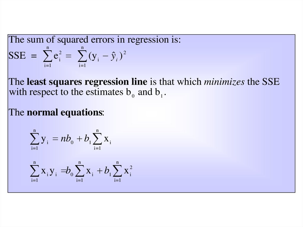
The sum of squared errors in regression is:
n
n
SSE = e (y i y i ) 2
2
i
i=1
i=1
The least squares regression line is that which minimizes the SSE
with respect to the estimates b 0 and b 1 .
The normal equations:
n
n
y nb b x
i
0
1
i=1
i
i=1
n
n
n
x y b x b x
i
i=1
i
0
i
i=1
1
i=1
2
i

39. Coefficient Equations

• Prediction equation
yˆi ˆ0 ˆ1 xi
• Sample slope
SS xy xi x yi y
ˆ1
2
SS xx
x
x
i
• Sample Y - intercept
ˆ0 y ˆ1x
39

40. Using the Equation

•Method of Least squares leads to that the intercept is 18.354
and the slope is 3.879.
–How do we predict the selling price of a house of 16,5 square meter?
• Plug in the value 16.50 in the regression equation and get predicted selling
price = 18.354 + 3.879× (16.50) = 82.357.
• Translate to a dollar amount, i.e., $82,357. This is the estimate you have of
the selling price of this house, that is, without any further information
about the house (e.g., neighborhood, number of rooms, lot size, age, etc.).
•Analyzing a Regression
•Estimating the Standard Error
–From the assumptions about the error, the magnitude of should be a
good guide to the accuracy of a prediction.
–The number is a population parameter, so we cannot know for
certain what its value is.
–We therefore use an estimate s that is provided in the regression
output under the name “standard error of the estimate” or just
“standard error.”

41. Making Predictions

•The estimate s is calculated by (SSE/(n-2))1/2.
–The reason why we divide by n - 2 and not n - 1 has to do with the
degrees of freedom issue.
–The value of s gives us some idea of the standard deviation of the
errors if the model is used to estimate selling prices. In addition, we
will make use of the normality assumption to help us make
assessments of a prediction.
•Suppose a house occupies 200 sq m. How do we predict the
selling price?
–prediction interval: This is used if our goal is to determine a 95%
confidence interval on the actual selling price of the house. A 95%
prediction interval for the actual selling price is given by
(18.354 + 3.879× 20 ) t(n - 2, 0.025)s = 95.94 26.8
–confidence interval: This is used if our goal is to determine a 95%
confidence interval on the mean selling price of all houses of this size
(200 square m). (E[Y|X = x])
It is 95,940 t(n - 2, 0.025)s /√n = 95.94 6.7 .
–In the above examples use the t distribution with n - 2 degrees of
freedom. If n - 2 30 then the standard normal distribution can be used
instead.

42. Making Inferences about Coefficients

•To assess the accuracy of the model, it involves determining
whether a particular variable like house size has any effect
on the selling price.
–Suppose that when a regression line is drawn it produces a horizontal
line. This means the selling price of the house is unaffected by the size
of the house.
–A horizontal line has a slope of 0, so when no linear relationship exists
between an independent variable and the dependent variable we
should expect to get 1 = 0.
–But of course, we only observe estimate of 1, which might only be
“close” to zero. To systematically determine when 1 might in fact be
zero, we will make inferences about it using our estimate , specifically,
we will do hypothesis tests and build confidence intervals.
•Testing 1, we can test any of the following:
–H0 : 1 = 0 versus HA : 1 0
–H0 : 1 0 versus HA : 1 < 0
–H0 : 1 0 versus HA : 1 > 0
• In each case, the null hypothesis can be reduced to H0: 1 = 0.
The test statistic in each case is ˆ1 0 / s ˆ
1

43. Example

•Can we conclude at the 1% level of significance that the size
of a house is linearly related to its selling price? Test H0 : 1 =
0 versus HA : 1 0
–Note this is a two-sided test, we are interested in whether there is any
relationship at all between price and size.
–Calculate T = (3.879 - 0) / 0.794 = 4.88.
–That is, we are 4.88 standard deviations from 0. So at the 1% level
(corresponding to thresholds t(13, 0.005) = 3.012), we reject H0.
–There is sufficient evidence to conclude that house size does linearly
affect selling price.
•To get a p-value on this we would need to look up 4.88
inside the t-table.
–It is 0.00024 or 0.024%; very small indeed.
•A 95% confidence interval for 1 is given by ˆ1 t( n 2,0.025) s ˆ1
–For this example: It is 3.879 (2.160)(0.794) = 3.879 1.715.
–Using the 15 data points, we are 95% confident that every extra square
foot increases the price of the house by anywhere from $21.64 to
$55.94.

44. Method III: Measuring the Strength of the Linear Relationship

•Consider the following equation:
Yi -Y = (Yˆ - Y ) + ei.
–Squaring both sides and summing over all data points, and after a little
algebra, we get:
i (Yi -Y )2 = i (Yˆ -Y )2 + i ei2, which we usually rewrite as:
SST = SSR + SSE,
(2)
where SST = i (Yi - Y )2 , SSR = i (ˆY -Y )2 and SSE = i ei2.
–Interpretation:
•SST stands for the “total sum of squares” - this is essentially the total
variation in the data set, i.e., the total variation of selling prices.
•SSR stands for “sum of squares due to regression” - this is the squared
variation around the mean of the estimated selling prices. This is sometimes
called the total variation explained by the regression.
•SSE stands for “sum of squares due to error” - this is simply the sum of the
squared residuals, and it is the variation in the Y variable that remains
unexplained after taking into account the variable X.
–The interpretation of equation (2) is that the total variation in Y (SST) is
made up of two parts: the total variation explained by the regression
(SSR) and the remaining unexplained variation (SSE).

45. Regression Picture

yi
C
ŷi xi 0
A
B
y
B
A
y
C
yi
x
n
( y y)
i
i 1
2
n
( yˆ y )
i
i 1
2
n
( yˆ y )
i
A2
B2
C2
SStotal
Total squared distance of
observations from naïve mean
of y
Total variation
SSreg
SSresidual
Variability due to x (regression)
2
i
i 1
Distance from regression line to naïve mean of y
*Least squares estimation
gave us the line (β) that
minimized C2
R2=SSreg/SStotal
Variance around the regression line
Additional variability not explained
by x—what least squares method aims
to minimize

46. Regression Statistics

•Define R2 = SSR/SST = 1- SSE/SST
–The fraction of the total variation explained by the regression.
–R2 is a measure of the explanatory power of the model.
–Multiple-R = (R2)1/2 (in one variable case = |rXY|)
•According to the definition of R2, adding extraneous
explanatory variables will artificially inflate the R2.
–We must be careful in interpreting this number.
–Introducing extra variables can lead to spurious results and can
interfere with the proper estimation of slopes for the important
variables.
•In order to penalize an excess of variables, we consider the
adjusted R2, which is
adjusted R2 = 1- [SSE/(n-k-1)]/[SST/(n-1)] .
Here n is the number of data and k is the number of
explanatory variables.
–The adjusted R2 thus divides numerator and denominator by their DF.

47. How to determine the value of used cars that customers trade in when purchasing new cars?

• Car dealers across North America use the “Red Book” to help them
determine the value of used cars that their customers trade in when
purchasing new cars.
–The book, which is published monthly, lists average trade-in values for all
basic models of North American, Japanese and European cars.
–These averages are determined on the basis of the amounts paid at recent
used-car auctions.
–The book indicates alternative values of each car model according to its
condition and optional features, but it does not inform dealers how the
odometer reading affects the trade in value.
• Question: In an experiment to determine whether the odometer
reading should be included in the Red Book, an interested buyer of
used cars randomly selects ten 3-year-old cars of the same make,
condition, and optional features.
–The trade-in value and mileage for each car are shown in the following table.

48. Data

Odometer Reading(1,000 miles) 59 92 61 72 52 67 88 62 95 83
Trade-in Value ($100s)
37 41 43 39 41 39 35 40 29 33
• Run the regression, with Trade-in Value as the dependent variable
(Y) and Odometer Reading as the independent variable (X). The
output appears on the following page.
•Regression Statistics
– Multiple R = 0.893, R2 = 0.798, Adjusted R2 = 0.773 Standard Error =
2.178
– Analysis of Variance
df
SS
MS
F
Significance F
Regression
1 150.14
150.14 31.64
0.000
Residual
Total
– Testing
Intercept
x
8
9
37.96
188.10
4.74
Coeff.
Stnd Error
t-Stat
P-value
56.205
-0.26682
3.535
0.04743
15.90
-5.63
0.000
0.000

49. F and F-significance

•F is a test statistic testing whether the estimated model is
meaningful; i.e., statistically significant.
–F =MSR/MSE
–A large F or a small p-value (or F-significance) implies that the model
is significant.
–It is unusual not to reject this null hypothesis.

50. Salary-budget Example

•A large corporation is concerned about maintaining parity in
salary levels across different divisions.
–As a rough guide, it determines that managers responsible for
comparable budgets in different divisions should have comparable
compensation.
•Data Analysis: The following is a list of salary levels for 20
managers and the sizes of the budgets they manage.
–salary<- c(59.0,67.4,50.4,83.2,105.6,86.0,74.4,52.2,82.6,59.0,44.8,111.4,122.4,
82.6,57.0,70.8,54.6,111.0,86.2,79.0)
–budget<- c(3.5,5.0,2.5,6.0,7.5,4.5,6.0,4.0,4.5,5.0,2.5,12.5,9.0,7.5,6.0, 5.0,3.0,
8.5, 7.5, 6.5)
–Salary Y ($1000s)
–Budget X ($100,000s)

51. Salary-budget Example

• Want to fit a straight line to this data.
– The slope of this line gives the marginal increase in salary with respect to
increase in budget responsibility.
– The regression equation is SALARY = 31.9 + 7.73 BUDGET
– Each additional $100,000 of budget responsibility translates to an expected
additional salary of $7,730.
– If we wanted to know the average salary corresponding to a budget of 6.0, we
get a salary of 31.9 + 7.73(6.0) = 78.28.
• Why is the least squares criterion the correct principle to follow?
• Assumptions Underlying Least Squares
– The errors 1,…, n are independent of the values of X1,…,Xn.
– The errors have expected value zero; i.e., E[ i] = 0.
– All the errors have the same variance: Var[ i] = 2, for all i = 1,…,n.
– The errors are uncorrelated; i.e., Corr[ i, j] = 0 if i j.
• The first two assumptions imply that E[Y|X = x] = 0 + 1x.
– Do we necessarily believe that the variability in salary levels among
managers with large budgets is the same as the variability among managers
with small budgets?

52. How do we evaluate and use the regression line?

• Evaluate the explanatory power of a model.
– Without using X, how do we predict Y?
– Determine how much of the variability in Y values is explained by the X.
• Measure variability using sums of squared quantities.
• The ANOVA table.
– ANOVA is short for analysis of variance.
– This table breaks down the total variability into the explained and
unexplained parts.
– Total SS (9535.8) measures the total variability in the salary levels.
• Without using x, we will use sample mean to do prediction.
– The Regression SS (6884.7) is the explained variation.
• It measures how much variability is explained by differences in budgets.
– Error SS (2651.1) is the unexplained variation.
• This reflects differences in salary levels that cannot be attributed to differences in
budget responsibilities.
– The explained and unexplained variation sum to the Total SS.
• R-squared: R-sq = SSR/SST = 6884.7/9538.8 = 72:2%