Vasileios Zarikas Associate Professor School of Engineering and Digital Sciences Nazarbayev University

1.25M

Категория:

Образование

School of Engineering and Digital Sciences

1. Vasileios Zarikas Associate Professor School of Engineering and Digital Sciences Nazarbayev University

Engineering
Mathematics
III
Vasileios Zarikas
Associate Professor
School of Engineering and Digital Sciences
Nazarbayev University
Finite Mathematics: An Applied Approach by Michael Sullivan
Copyright 2011 by John Wiley & Sons. All rights reserved.

2.

1.3
Section 1.3 p2
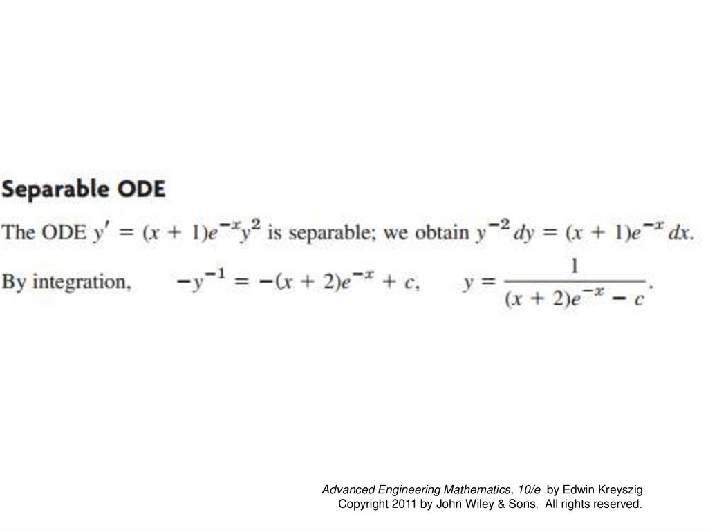
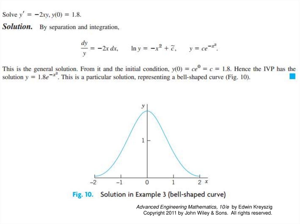
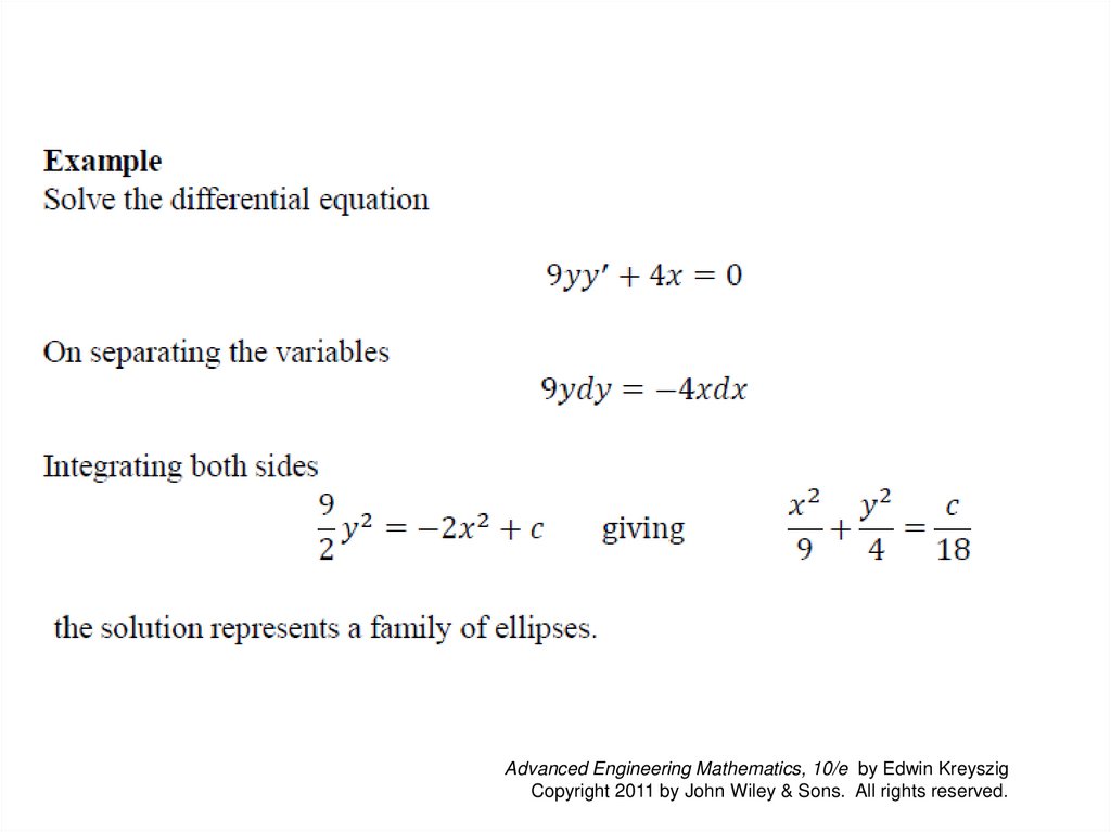
Separable ODEs. Modeling
Advanced Engineering Mathematics, 10/e by Edwin Kreyszig
Copyright 2011 by John Wiley & Sons. All rights reserved.

3.

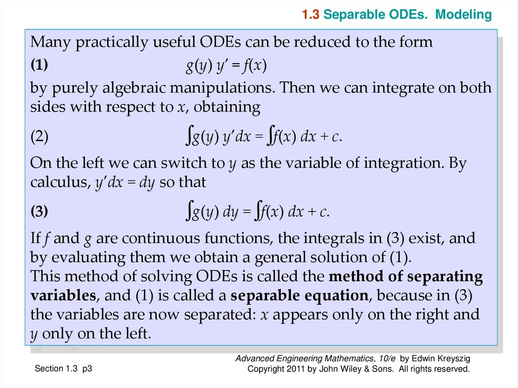
1.3 Separable ODEs. Modeling
Many practically useful ODEs can be reduced to the form
(1)
g(y) y’ = f(x)
by purely algebraic manipulations. Then we can integrate on both
sides with respect to x, obtaining
(2)
∫g(y) y’dx = ∫f(x) dx + c.
On the left we can switch to y as the variable of integration. By
calculus, y’dx = dy so that
(3)
∫g(y) dy = ∫f(x) dx + c.
If f and g are continuous functions, the integrals in (3) exist, and
by evaluating them we obtain a general solution of (1).
This method of solving ODEs is called the method of separating
variables, and (1) is called a separable equation, because in (3)
the variables are now separated: x appears only on the right and
y only on the left.
Section 1.3 p3
Advanced Engineering Mathematics, 10/e by Edwin Kreyszig
Copyright 2011 by John Wiley & Sons. All rights reserved.

4.

Advanced Engineering Mathematics, 10/e by Edwin Kreyszig
Copyright 2011 by John Wiley & Sons. All rights reserved.

5.

Advanced Engineering Mathematics, 10/e by Edwin Kreyszig
Copyright 2011 by John Wiley & Sons. All rights reserved.

6.

Advanced Engineering Mathematics, 10/e by Edwin Kreyszig
Copyright 2011 by John Wiley & Sons. All rights reserved.

7.

Advanced Engineering Mathematics, 10/e by Edwin Kreyszig
Copyright 2011 by John Wiley & Sons. All rights reserved.

8.

Advanced Engineering Mathematics, 10/e by Edwin Kreyszig
Copyright 2011 by John Wiley & Sons. All rights reserved.

9.

Advanced Engineering Mathematics, 10/e by Edwin Kreyszig
Copyright 2011 by John Wiley & Sons. All rights reserved.

10.

Advanced Engineering Mathematics, 10/e by Edwin Kreyszig
Copyright 2011 by John Wiley & Sons. All rights reserved.

11.

Advanced Engineering Mathematics, 10/e by Edwin Kreyszig
Copyright 2011 by John Wiley & Sons. All rights reserved.

12.

Advanced Engineering Mathematics, 10/e by Edwin Kreyszig
Copyright 2011 by John Wiley & Sons. All rights reserved.

13.

Advanced Engineering Mathematics, 10/e by Edwin Kreyszig
Copyright 2011 by John Wiley & Sons. All rights reserved.

14.

1.3 Separable ODEs. Modeling
EXAMPLE 5
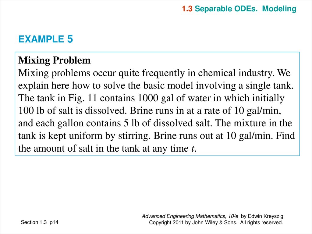
Mixing Problem
Mixing problems occur quite frequently in chemical industry. We
explain here how to solve the basic model involving a single tank.
The tank in Fig. 11 contains 1000 gal of water in which initially
100 lb of salt is dissolved. Brine runs in at a rate of 10 gal/min,
and each gallon contains 5 lb of dissolved salt. The mixture in the
tank is kept uniform by stirring. Brine runs out at 10 gal/min. Find
the amount of salt in the tank at any time t.
Section 1.3 p14
Advanced Engineering Mathematics, 10/e by Edwin Kreyszig
Copyright 2011 by John Wiley & Sons. All rights reserved.

15.

1.3 Separable ODEs. Modeling
EXAMPLE 5 (continued)
Solution.
Step 1. Setting up a model.
Let y(t) denote the amount of salt in the tank at time t. Its
time rate of change is
y’ = Salt inflow rate - Salt outflow rate
Balance law.
5 lb times 10 gal gives an inflow of 50 lb of salt. Now, the
outflow is 10 gal of brine.
This is 10/1000 = 0.01( = 1%) of the total brine content in the
tank, hence 0.01 of the salt content y(t), that is, 0.01 y(t) .
Thus the model is the ODE
(4)
y’ = 50 − 0.01y = −0.01(y − 5000).
Section 1.3 p15
Advanced Engineering Mathematics, 10/e by Edwin Kreyszig
Copyright 2011 by John Wiley & Sons. All rights reserved.

16.

1.3 Separable ODEs. Modeling
EXAMPLE 5 (continued)
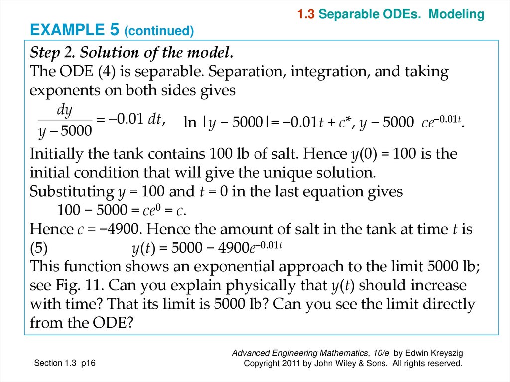
Step 2. Solution of the model.
The ODE (4) is separable. Separation, integration, and taking
exponents on both sides gives
dy
0.01 dt , ln |y − 5000|= −0.01t + c*, y − 5000 ce−0.01t.
y 5000
Initially the tank contains 100 lb of salt. Hence y(0) = 100 is the
initial condition that will give the unique solution.
Substituting y = 100 and t = 0 in the last equation gives
100 − 5000 = ce0 = c.
Hence c = −4900. Hence the amount of salt in the tank at time t is
(5)
y(t) = 5000 − 4900e−0.01t
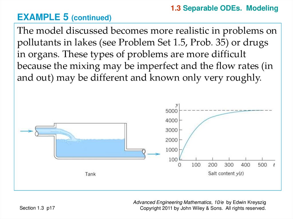
This function shows an exponential approach to the limit 5000 lb;
see Fig. 11. Can you explain physically that y(t) should increase
with time? That its limit is 5000 lb? Can you see the limit directly
from the ODE?
Section 1.3 p16
Advanced Engineering Mathematics, 10/e by Edwin Kreyszig
Copyright 2011 by John Wiley & Sons. All rights reserved.

17.

1.3 Separable ODEs. Modeling
EXAMPLE 5 (continued)
The model discussed becomes more realistic in problems on
pollutants in lakes (see Problem Set 1.5, Prob. 35) or drugs
in organs. These types of problems are more difficult
because the mixing may be imperfect and the flow rates (in
and out) may be different and known only very roughly.
Section 1.3 p17
Advanced Engineering Mathematics, 10/e by Edwin Kreyszig
Copyright 2011 by John Wiley & Sons. All rights reserved.

18.

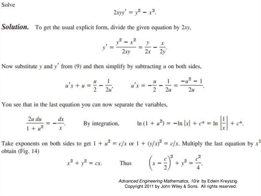
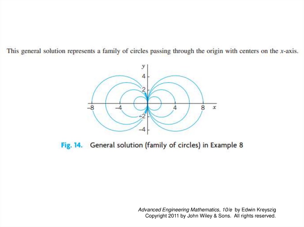
1.3 Separable ODEs. Modeling
Extended Method:
Reduction to Separable Form
Certain non separable ODEs can be made separable by
transformations that introduce for y a new unknown
function. We discuss this technique for a class of ODEs of
practical importance, namely, for equations
y
y ' f .
(8)
x
Here, f is any (differentiable) function of y/x such as
sin (y/x), (y/x)4, and so on. (Such an ODE is sometimes
called a homogeneous ODE, a term we shall not use but
reserve for a more important purpose in Sec. 1.5.)
Section 1.3 p18
Advanced Engineering Mathematics, 10/e by Edwin Kreyszig
Copyright 2011 by John Wiley & Sons. All rights reserved.

19.

1.3 Separable ODEs. Modeling
Extended Method:
Reduction to Separable Form (continued)
The form of such an ODE suggests that we set y/x = u; thus,
(9)
y = ux
and by product differentiation
y’ = u’x + u.
Substitution into y’ = f(y/x) then gives u’x + u = f (u)
or u’x = f(u) − u. We see that if f(u) − u ≠ 0, this can be
separated:
du
dx
.
(10)
f (u) u x
Section 1.3 p19
Advanced Engineering Mathematics, 10/e by Edwin Kreyszig
Copyright 2011 by John Wiley & Sons. All rights reserved.

20.

Advanced Engineering Mathematics, 10/e by Edwin Kreyszig
Copyright 2011 by John Wiley & Sons. All rights reserved.

21.

Advanced Engineering Mathematics, 10/e by Edwin Kreyszig
Copyright 2011 by John Wiley & Sons. All rights reserved.

22.

Advanced Engineering Mathematics, 10/e by Edwin Kreyszig
Copyright 2011 by John Wiley & Sons. All rights reserved.

23.

Advanced Engineering Mathematics, 10/e by Edwin Kreyszig
Copyright 2011 by John Wiley & Sons. All rights reserved.

24.

1.4
Section 1.4 p24
Exact ODEs. Integrating
Factors
Advanced Engineering Mathematics, 10/e by Edwin Kreyszig
Copyright 2011 by John Wiley & Sons. All rights reserved.

25.

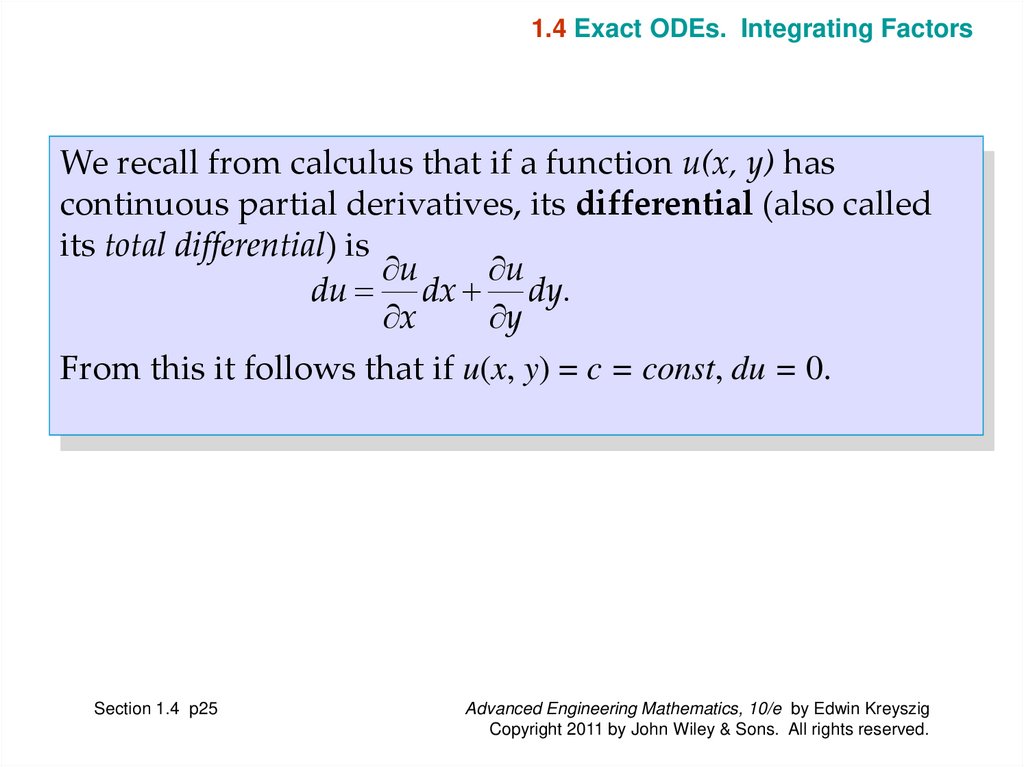
1.4 Exact ODEs. Integrating Factors
We recall from calculus that if a function u(x, y) has
continuous partial derivatives, its differential (also called
its total differential) is
u
u
du dx dy.
x
y
From this it follows that if u(x, y) = c = const, du = 0.
Section 1.4 p25
Advanced Engineering Mathematics, 10/e by Edwin Kreyszig
Copyright 2011 by John Wiley & Sons. All rights reserved.

26.

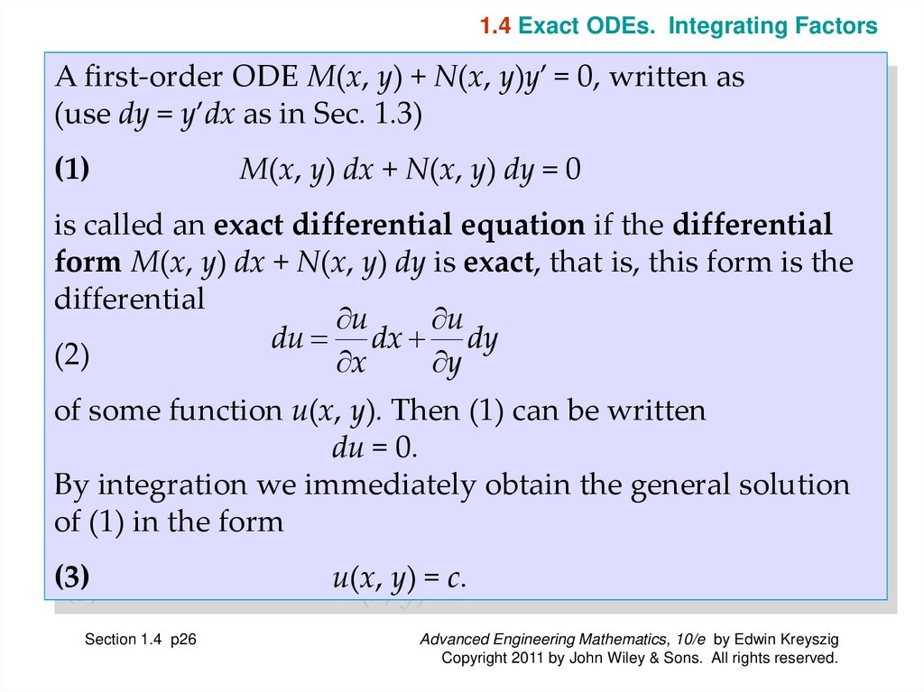
1.4 Exact ODEs. Integrating Factors
A first-order ODE M(x, y) + N(x, y)y’ = 0, written as
(use dy = y’dx as in Sec. 1.3)
(1)
M(x, y) dx + N(x, y) dy = 0
is called an exact differential equation if the differential
form M(x, y) dx + N(x, y) dy is exact, that is, this form is the
differential
u
u
du dx dy
(2)
x
y
of some function u(x, y). Then (1) can be written
du = 0.
By integration we immediately obtain the general solution
of (1) in the form
(3)
Section 1.4 p26
u(x, y) = c.
Advanced Engineering Mathematics, 10/e by Edwin Kreyszig
Copyright 2011 by John Wiley & Sons. All rights reserved.

27.

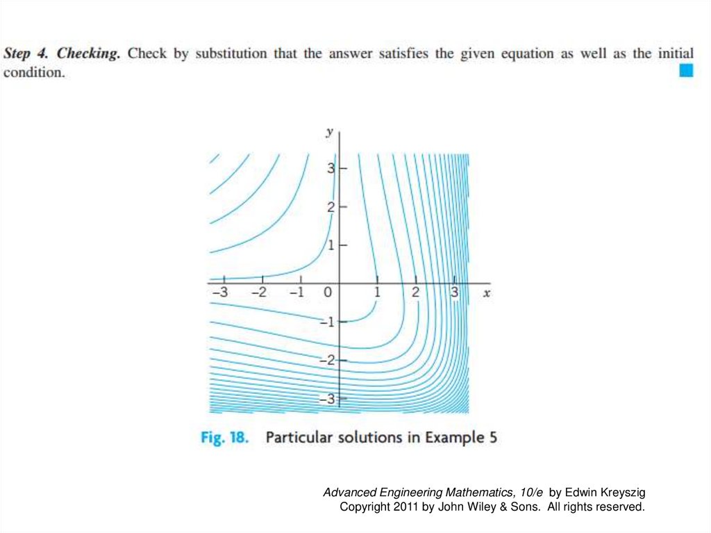
1.4 Exact ODEs. Integrating Factors
This is called an implicit solution, in contrast to a solution
y = h(x) as defined in Sec. 1.1, which is also called an explicit
solution, for distinction. Sometimes an implicit solution can
be converted to explicit form. (Do this for x2 + y2 = 1.) If this
is not possible, your CAS may graph a figure of the contour
lines (3) of the function u(x, y) and help you in
understanding the solution.
Comparing (1) and (2), we see that (1) is an exact
differential equation if there is some function u(x, y) such
that
u
u
M
(4)
(a)
(b)
N.
x
y
From this we can derive a formula for checking whether (1)
is exact or not, as follows.
Section 1.4 p27
Advanced Engineering Mathematics, 10/e by Edwin Kreyszig
Copyright 2011 by John Wiley & Sons. All rights reserved.

28.

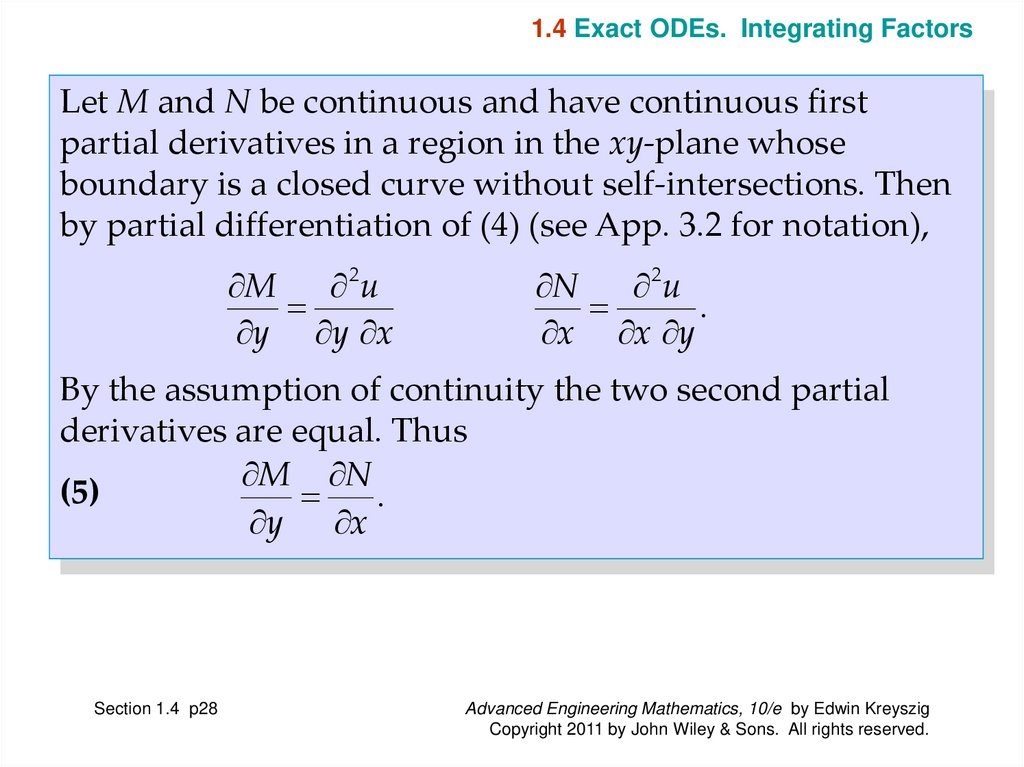
1.4 Exact ODEs. Integrating Factors
Let M and N be continuous and have continuous first
partial derivatives in a region in the xy-plane whose
boundary is a closed curve without self-intersections. Then
by partial differentiation of (4) (see App. 3.2 for notation),
M
2u
y y x
N
2u
.
x x y
By the assumption of continuity the two second partial
derivatives are equal. Thus
M N
(5)
.
y x
Section 1.4 p28
Advanced Engineering Mathematics, 10/e by Edwin Kreyszig
Copyright 2011 by John Wiley & Sons. All rights reserved.

29.

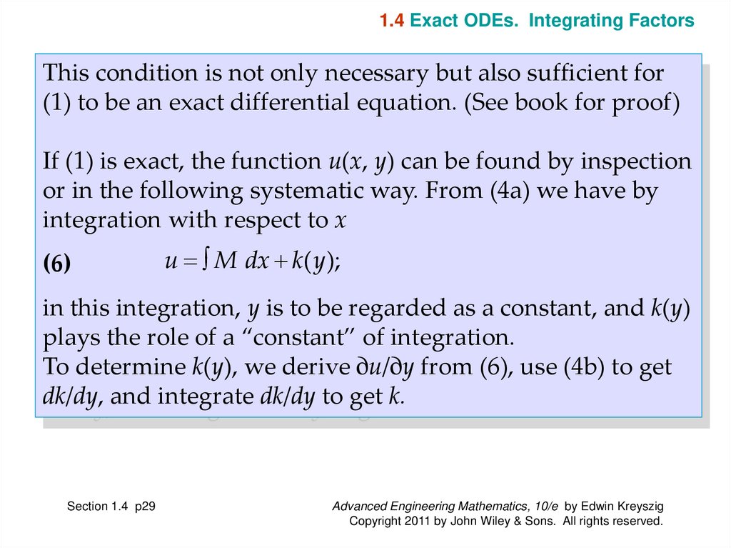
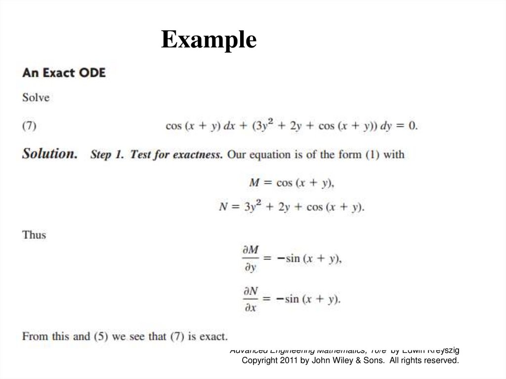
1.4 Exact ODEs. Integrating Factors
This condition is not only necessary but also sufficient for
(1) to be an exact differential equation. (See book for proof)
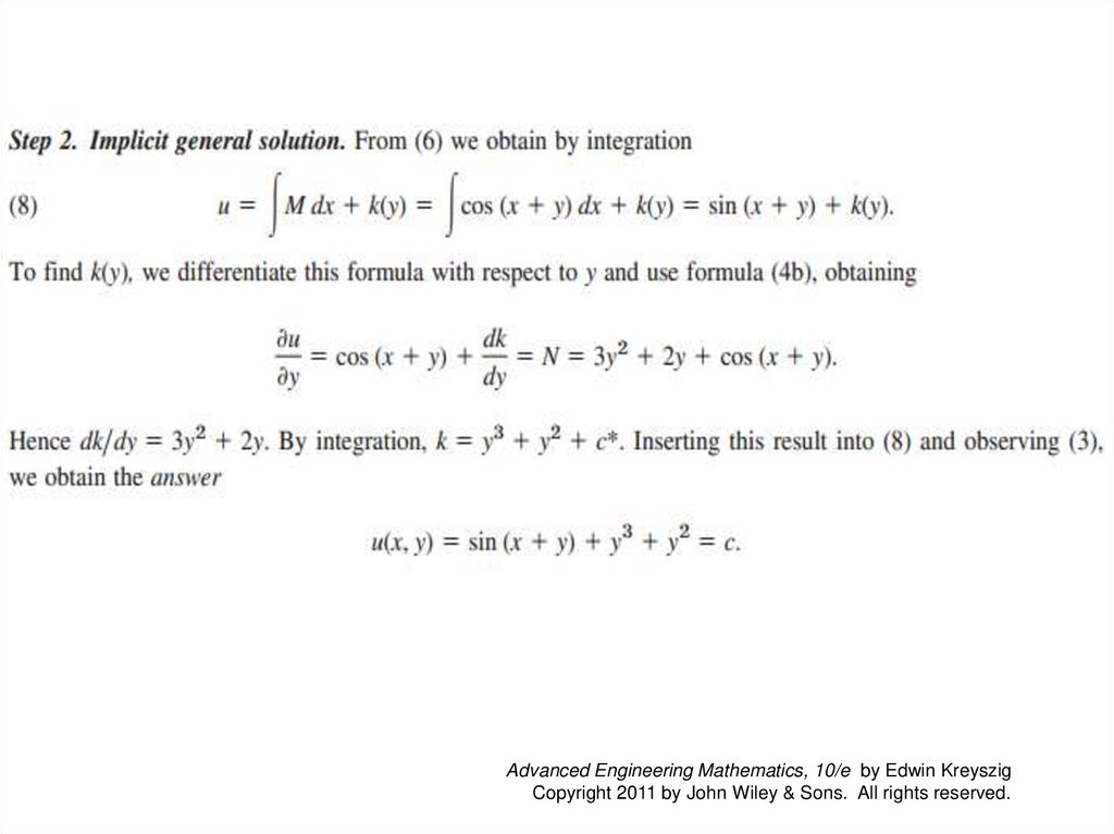
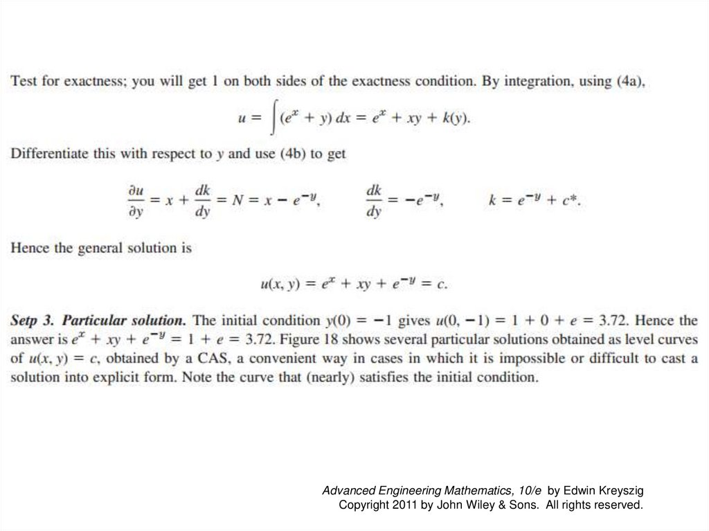
If (1) is exact, the function u(x, y) can be found by inspection
or in the following systematic way. From (4a) we have by
integration with respect to x
(6)
u M dx k( y);
in this integration, y is to be regarded as a constant, and k(y)
plays the role of a “constant” of integration.
To determine k(y), we derive ∂u/∂y from (6), use (4b) to get
dk/dy, and integrate dk/dy to get k.
Section 1.4 p29
Advanced Engineering Mathematics, 10/e by Edwin Kreyszig
Copyright 2011 by John Wiley & Sons. All rights reserved.

30.

31.

32.

33.

34.

35.

36.

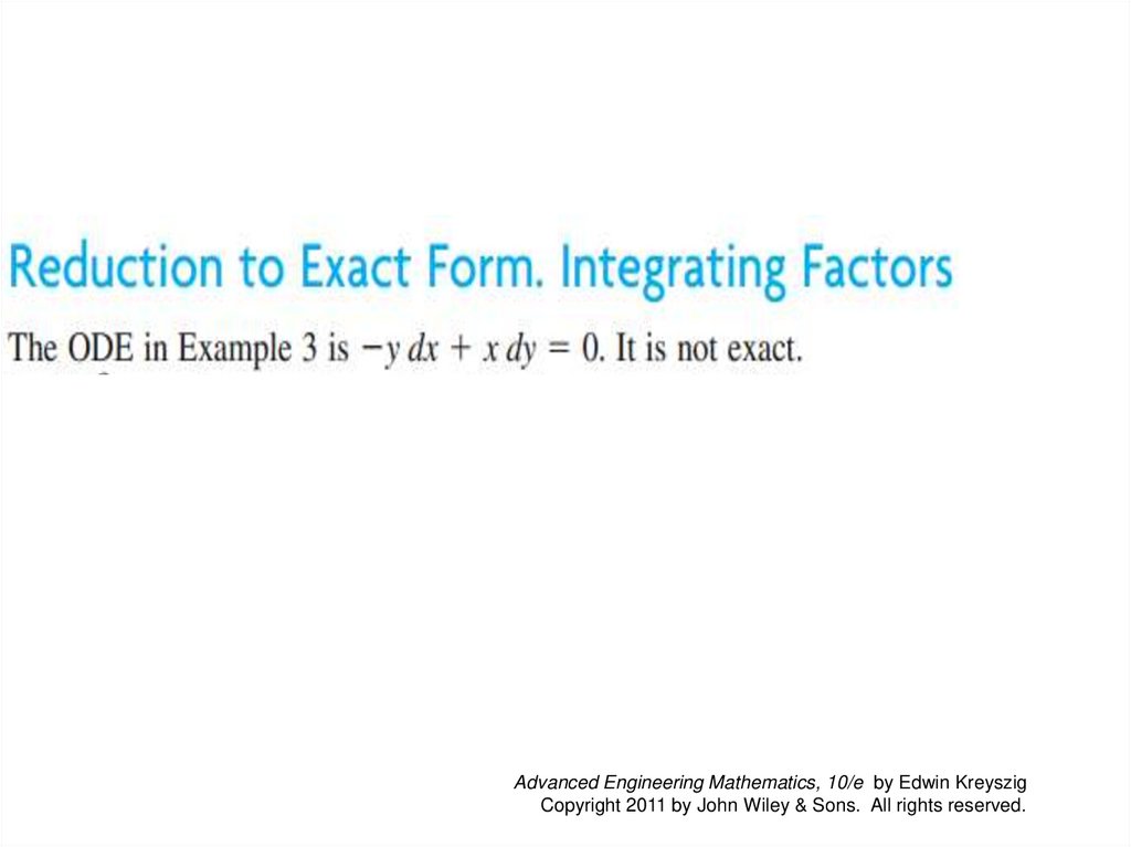
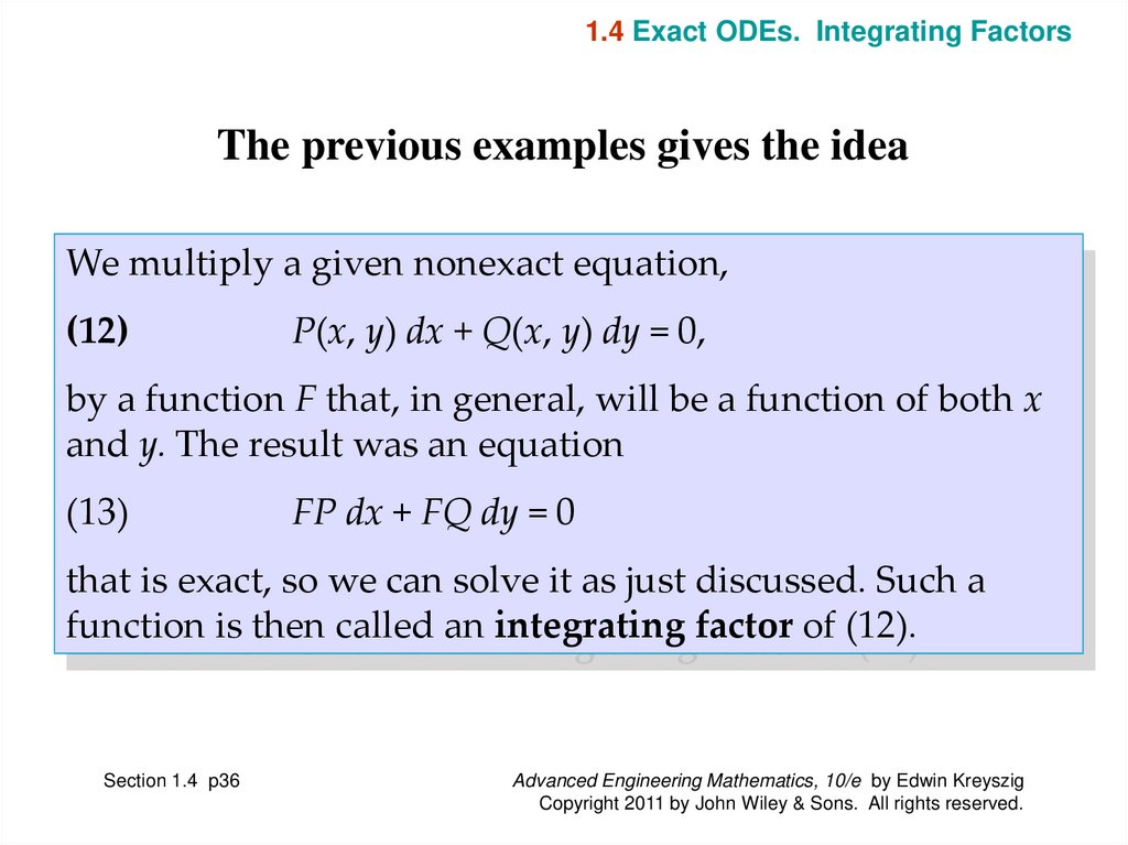
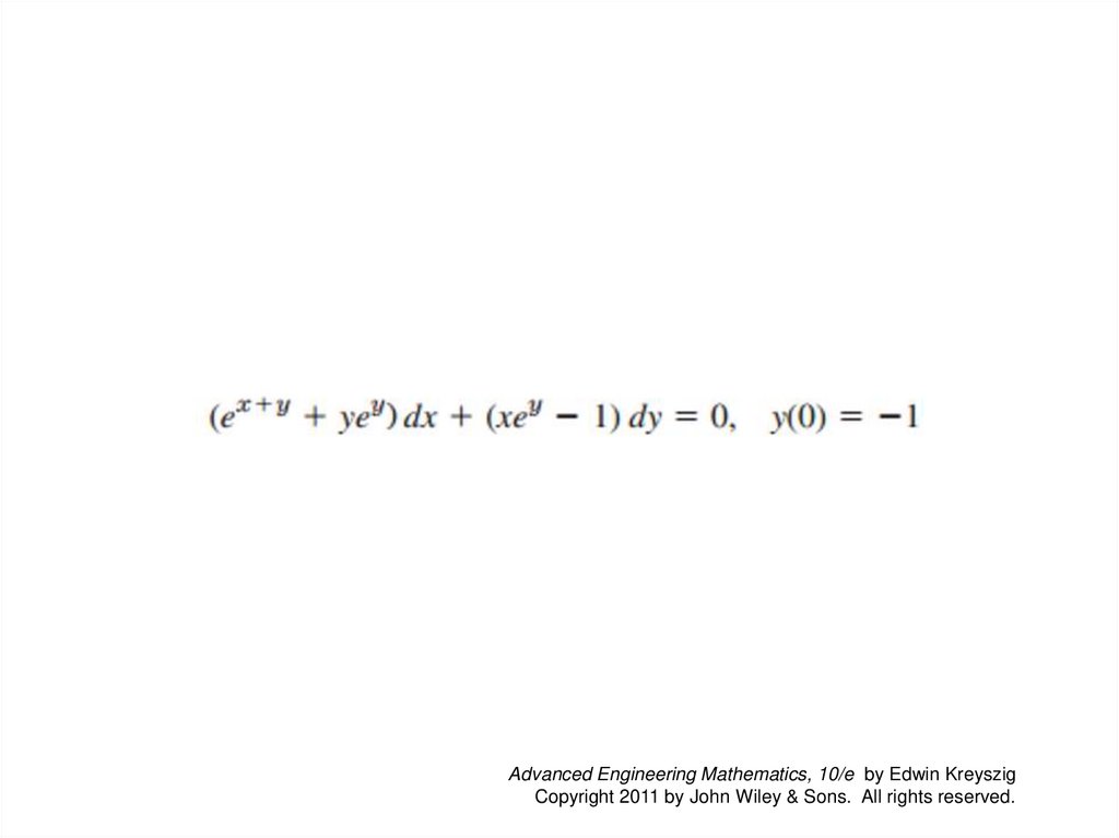
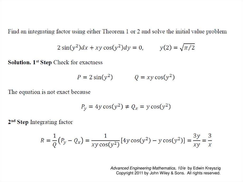
1.4 Exact ODEs. Integrating Factors
The previous examples gives the idea
We multiply a given nonexact equation,
(12)
P(x, y) dx + Q(x, y) dy = 0,
by a function F that, in general, will be a function of both x
and y. The result was an equation
(13)
FP dx + FQ dy = 0
that is exact, so we can solve it as just discussed. Such a
function is then called an integrating factor of (12).
Section 1.4 p36
Advanced Engineering Mathematics, 10/e by Edwin Kreyszig
Copyright 2011 by John Wiley & Sons. All rights reserved.

37.

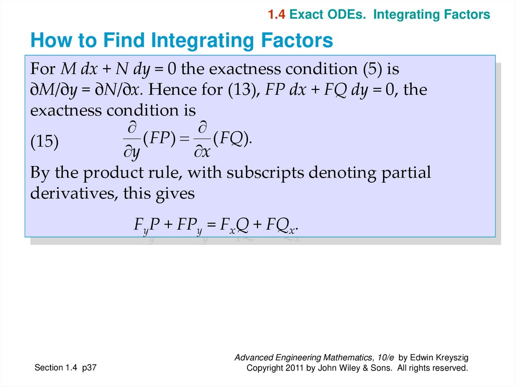
1.4 Exact ODEs. Integrating Factors
How to Find Integrating Factors
For M dx + N dy = 0 the exactness condition (5) is
∂M/∂y = ∂N/∂x. Hence for (13), FP dx + FQ dy = 0, the
exactness condition is
( FP) ( FQ).
(15)
y
x
By the product rule, with subscripts denoting partial
derivatives, this gives
FyP + FPy = FxQ + FQx.
Section 1.4 p37
Advanced Engineering Mathematics, 10/e by Edwin Kreyszig
Copyright 2011 by John Wiley & Sons. All rights reserved.

38.

1.4 Exact ODEs. Integrating Factors
How to Find Integrating Factors (continued)
Let F = F(x). Then Fy = 0, and Fx = F’ = dF/dx, so that (15)
becomes
FPy = F’Q + FQx.
Dividing by FQ and reshuffling terms, we have
1 dF
1 P Q
(16)
R,
where
R
.
F dx
Q y x
Section 1.4 p38
Advanced Engineering Mathematics, 10/e by Edwin Kreyszig
Copyright 2011 by John Wiley & Sons. All rights reserved.

39.

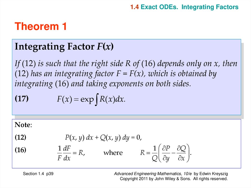
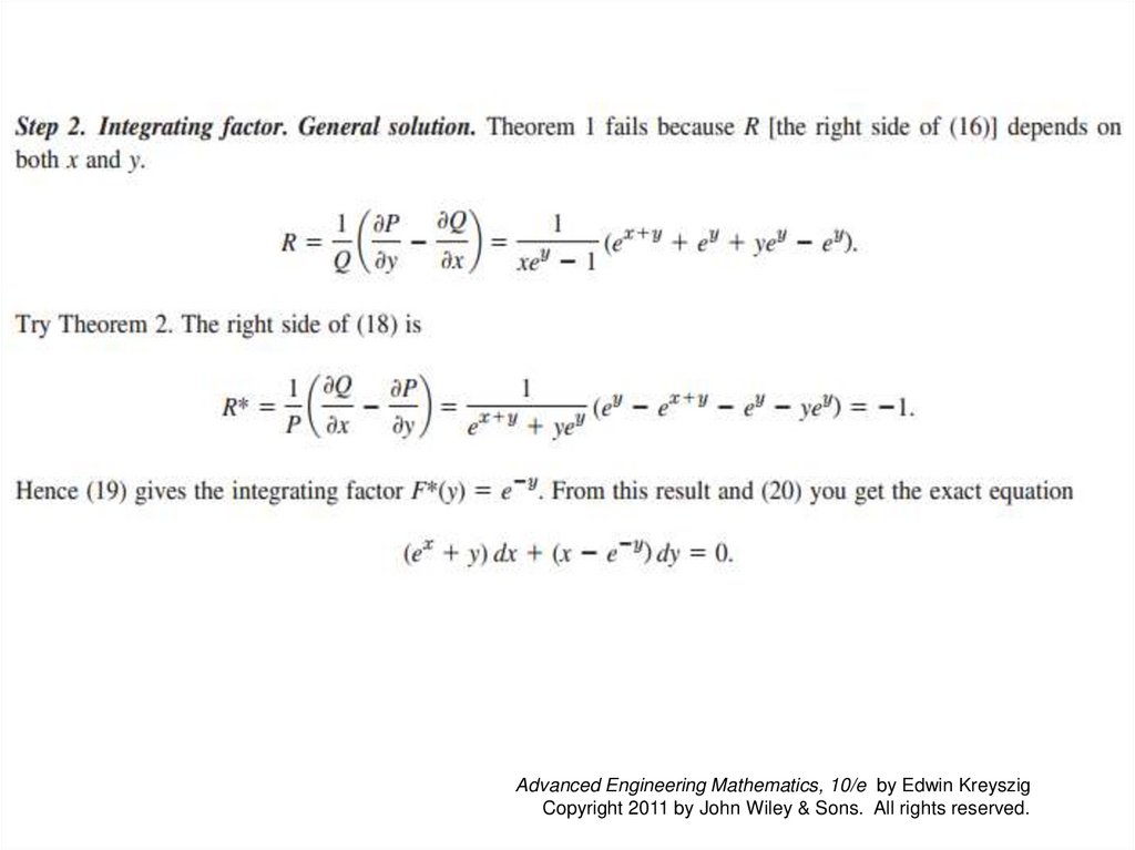
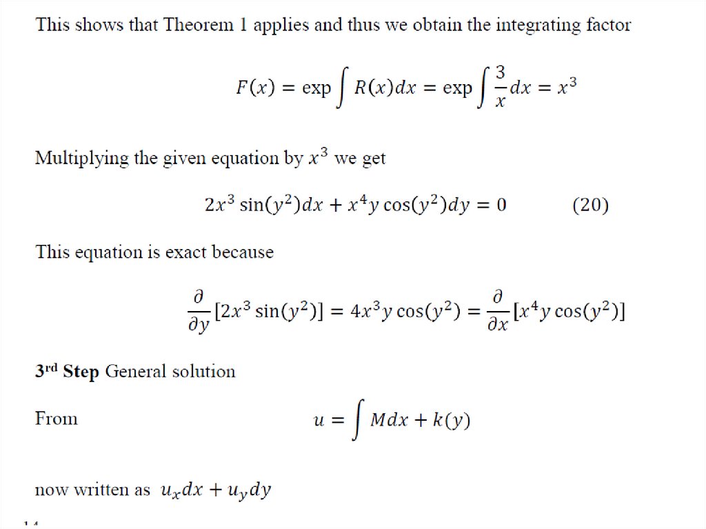
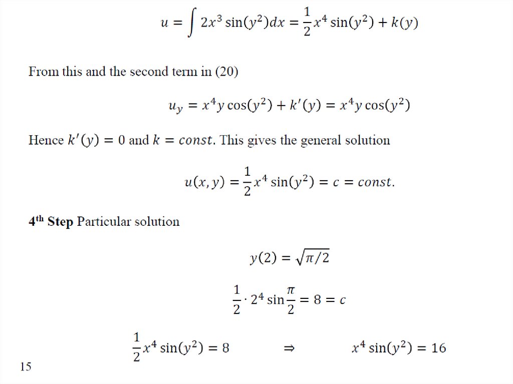
1.4 Exact ODEs. Integrating Factors
Theorem 1
Integrating Factor F(x)
If (12) is such that the right side R of (16) depends only on x, then
(12) has an integrating factor F = F(x), which is obtained by
integrating (16) and taking exponents on both sides.
(17)
F( x) exp R( x)dx.
Note:
(12)
(16)
Section 1.4 p39
P(x, y) dx + Q(x, y) dy = 0,
1 dF
R,
F dx
where
R
1 P Q
.
Q y x
Advanced Engineering Mathematics, 10/e by Edwin Kreyszig
Copyright 2011 by John Wiley & Sons. All rights reserved.

40.

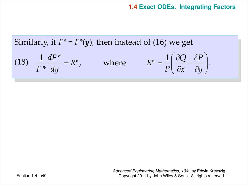
1.4 Exact ODEs. Integrating Factors
Similarly, if F* = F*(y), then instead of (16) we get
1 dF *
(18)
R*,
F * dy
Section 1.4 p40
where
1 Q P
R*
.
P x y
Advanced Engineering Mathematics, 10/e by Edwin Kreyszig
Copyright 2011 by John Wiley & Sons. All rights reserved.

41.

1.4 Exact ODEs. Integrating Factors
Theorem 2
Integrating Factor F*(y)
If (12) is such that the right side R* of (18) depends only on y,
then (12) has an integrating factor F* = F*(y), which is obtained
from (18) and taking exponents on both sides.
F *( y) exp R*( y)dy
(19)
Note:
(12)
(18)
P(x, y) dx + Q(x, y) dy = 0,
1 dF *
1 Q P
R*,
where
R*
.
F * dy
P x y
Section 1.4 p41
Advanced Engineering Mathematics, 10/e by Edwin Kreyszig
Copyright 2011 by John Wiley & Sons. All rights reserved.

42.

43.

44.

45.

46.

47.

48.

49.

50.

51.

1.5 Linear ODEs. Bernoulli Equation. Population Dynamics.
A first-order ODE is said to be linear if it can be brought
into the form
(1)
y’ + p(x)y = r(x),
by algebra, and nonlinear if it cannot be brought into this
form.
Section 1.5 p51
Advanced Engineering Mathematics, 10/e by Edwin Kreyszig
Copyright 2011 by John Wiley & Sons. All rights reserved.

52.

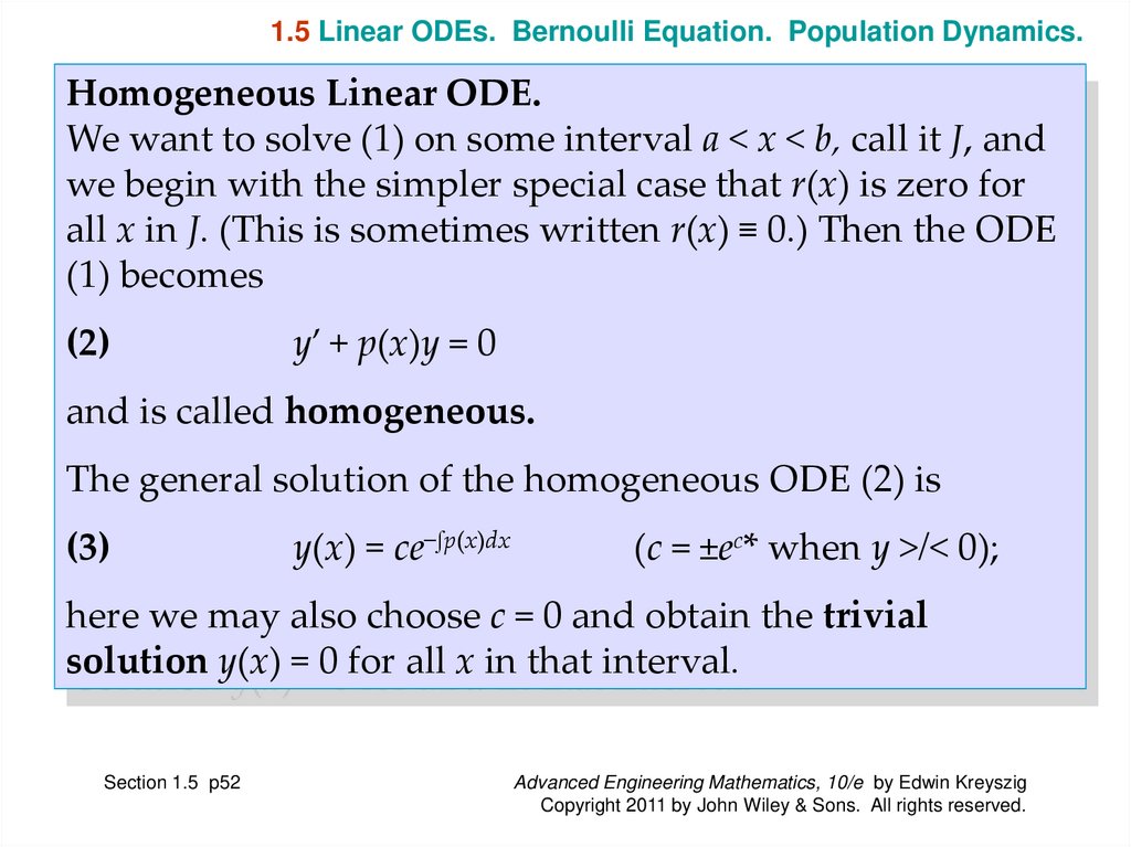
1.5 Linear ODEs. Bernoulli Equation. Population Dynamics.
Homogeneous Linear ODE.
We want to solve (1) on some interval a < x < b, call it J, and
we begin with the simpler special case that r(x) is zero for
all x in J. (This is sometimes written r(x) ≡ 0.) Then the ODE
(1) becomes
(2)
y’ + p(x)y = 0
and is called homogeneous.
The general solution of the homogeneous ODE (2) is
(3)
y(x) = ce−∫p(x)dx
(c = ±ec* when y >/< 0);
here we may also choose c = 0 and obtain the trivial
solution y(x) = 0 for all x in that interval.
Section 1.5 p52
Advanced Engineering Mathematics, 10/e by Edwin Kreyszig
Copyright 2011 by John Wiley & Sons. All rights reserved.

53.

1.5 Linear ODEs. Bernoulli Equation. Population Dynamics.
Nonhomogeneous Linear ODE
We now solve (1) in the case that r(x) in (1) is not everywhere zero
on the interval J considered. Then the ODE (1) is called
nonhomogeneous.
Solution of nonhomogeneous linear ODE (1):
(4)
y(x) = e−h(∫ehr dx + c),
h = ∫p(x) dx.
The structure of (4) is interesting. The only quantity depending
on a given initial condition is c. Accordingly, writing (4) as a sum
of two terms,
(4*)
y(x) = e−h∫ehr dx + c e−h,
we see the following:
(5) Total Output = Response to the Input r + Response to the
Initial Data.
Section 1.5 p53
Advanced Engineering Mathematics, 10/e by Edwin Kreyszig
Copyright 2011 by John Wiley & Sons. All rights reserved.

54.

55.

1.5 Linear ODEs. Bernoulli Equation. Population Dynamics.
EXAMPLE 1
First-Order ODE, General Solution, Initial Value Problem
Solve the initial value problem
y’ + y tan x = sin 2x,
y(0) = 1.
Solution.
Here p = tan x, r = sin 2x = 2 sin x cos x and
h = ∫p dx = ∫tan x dx = ln|sec x|.
From this we see that in (4),
eh = sec x, e−h = cos x, ehr = (sec x)(2 sin x cos x) = 2 sin x,
and the general solution of our equation is
y(x) = cos x (2 ∫sin x dx + c) = c cos x − 2 cos2x.
From this and the initial condition, 1 = c · 1 − 2 · 12, thus c = 3 and
the solution of our initial value problem is y = 3 cos x - 2 cos2 x.
Here 3 cos x is the response to the initial data, and −2 cos2 x is the
response to the input sin 2x.
Section 1.5 p55
Advanced Engineering Mathematics, 10/e by Edwin Kreyszig
Copyright 2011 by John Wiley & Sons. All rights reserved.

56.

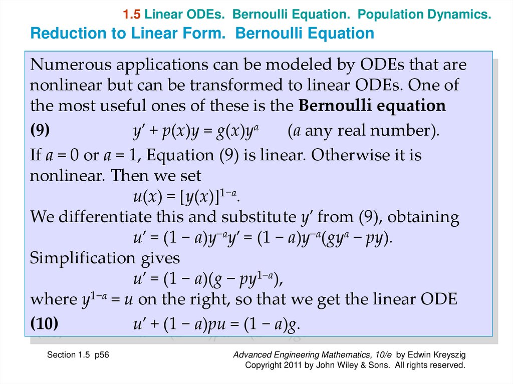
1.5 Linear ODEs. Bernoulli Equation. Population Dynamics.
Reduction to Linear Form. Bernoulli Equation
Numerous applications can be modeled by ODEs that are
nonlinear but can be transformed to linear ODEs. One of
the most useful ones of these is the Bernoulli equation
(9)
y’ + p(x)y = g(x)ya
(a any real number).
If a = 0 or a = 1, Equation (9) is linear. Otherwise it is
nonlinear. Then we set
u(x) = [y(x)]1−a.
We differentiate this and substitute y’ from (9), obtaining
u’ = (1 − a)y−ay’ = (1 − a)y−a(gya − py).
Simplification gives
u’ = (1 − a)(g − py1−a),
where y1−a = u on the right, so that we get the linear ODE
(10)
u’ + (1 − a)pu = (1 − a)g.
Section 1.5 p56
Advanced Engineering Mathematics, 10/e by Edwin Kreyszig
Copyright 2011 by John Wiley & Sons. All rights reserved.

57.

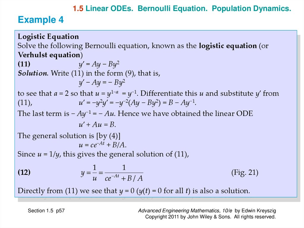
1.5 Linear ODEs. Bernoulli Equation. Population Dynamics.
Example 4
Logistic Equation
Solve the following Bernoulli equation, known as the logistic equation (or
Verhulst equation)
(11)
y’ = Ay − By2
Solution. Write (11) in the form (9), that is,
y’ − Ay = − By2
to see that a = 2 so that u = y1−a = y−1. Differentiate this u and substitute y’ from
(11),
u’ = −y2y’ = −y−2(Ay − By2) = B − Ay−1.
The last term is − Ay−1 = − Au. Hence we have obtained the linear ODE
u’ + Au = B.
The general solution is [by (4)]
u = ce−At + B/A.
Since u = 1/y, this gives the general solution of (11),
(12)
y
1
1
At
u ce B / A
(Fig. 21)
Directly from (11) we see that y = 0 (y(t) = 0 for all t) is also a solution.
Section 1.5 p57
Advanced Engineering Mathematics, 10/e by Edwin Kreyszig
Copyright 2011 by John Wiley & Sons. All rights reserved.

58.

1.5 Linear ODEs. Bernoulli Equation. Population Dynamics.
Example 4 (continued)
Section 1.5 p58
Advanced Engineering Mathematics, 10/e by Edwin Kreyszig
Copyright 2011 by John Wiley & Sons. All rights reserved.

59.

60.

SUMMARY OF CHAPTER
1
First-Order ODEs
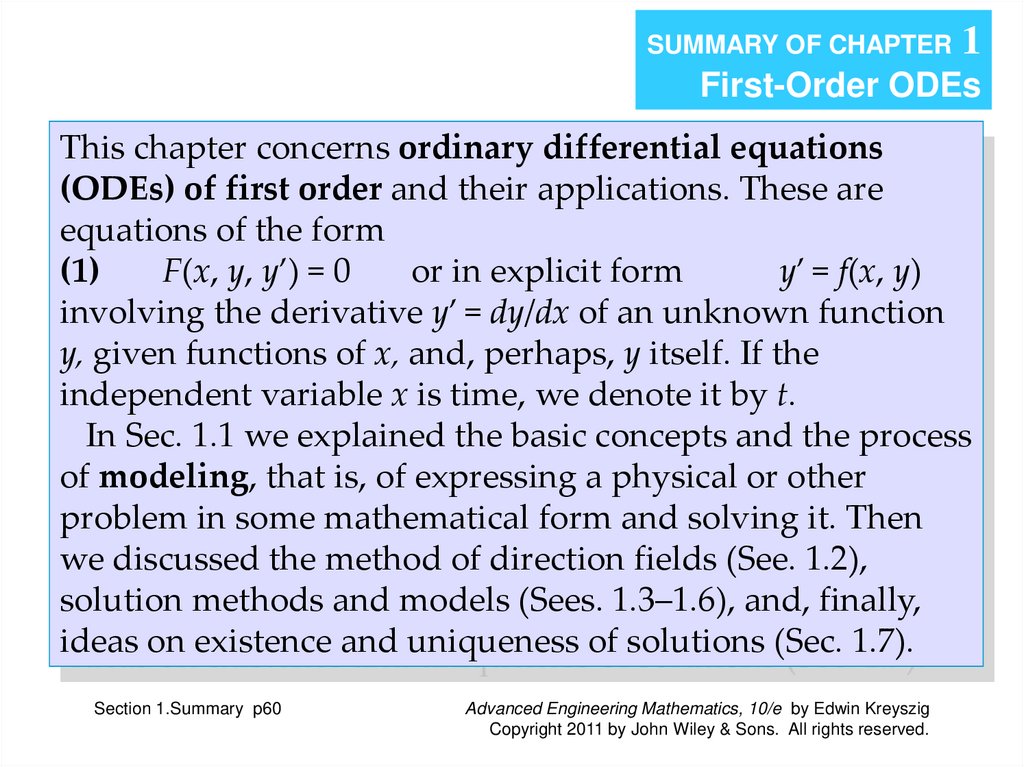
This chapter concerns ordinary differential equations
(ODEs) of first order and their applications. These are
equations of the form
(1)
F(x, y, y’) = 0
or in explicit form
y’ = f(x, y)
involving the derivative y’ = dy/dx of an unknown function
y, given functions of x, and, perhaps, y itself. If the
independent variable x is time, we denote it by t.
In Sec. 1.1 we explained the basic concepts and the process
of modeling, that is, of expressing a physical or other
problem in some mathematical form and solving it. Then
we discussed the method of direction fields (See. 1.2),
solution methods and models (Sees. 1.3–1.6), and, finally,
ideas on existence and uniqueness of solutions (Sec. 1.7).
Section 1.Summary p60
Advanced Engineering Mathematics, 10/e by Edwin Kreyszig
Copyright 2011 by John Wiley & Sons. All rights reserved.

61.

SUMMARY OF CHAPTER
1
First-Order ODEs
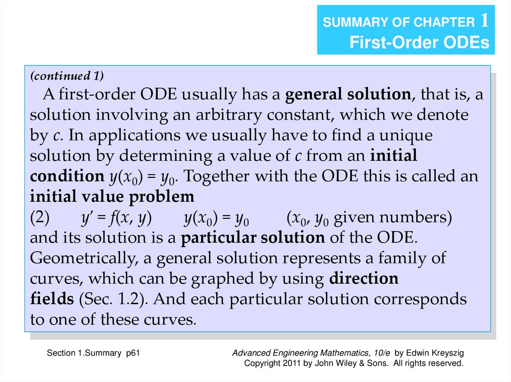
(continued 1)
A first-order ODE usually has a general solution, that is, a
solution involving an arbitrary constant, which we denote
by c. In applications we usually have to find a unique
solution by determining a value of c from an initial
condition y(x0) = y0. Together with the ODE this is called an
initial value problem
(2)
y’ = f(x, y)
y(x0) = y0
(x0, y0 given numbers)
and its solution is a particular solution of the ODE.
Geometrically, a general solution represents a family of
curves, which can be graphed by using direction
fields (Sec. 1.2). And each particular solution corresponds
to one of these curves.
Section 1.Summary p61
Advanced Engineering Mathematics, 10/e by Edwin Kreyszig
Copyright 2011 by John Wiley & Sons. All rights reserved.

62.

SUMMARY OF CHAPTER
1
First-Order ODEs
(continued 2)
A separable ODE is one that we can put into the form
(3)
g(y) dy = f (x) dx
(Sec. 1.3)
by algebraic manipulations (possibly combined with
transformations, such as y/x = u) and solve by integrating on
both sides.
An exact ODE is of the form
(4)
M(x, y) dx + N(x, y) dy = 0
(Sec. 1.4)
where M dx + N dy is the differential
du = ux dx + uy dy
of a function u(x, y), so that from du = 0 we immediately get the
implicit general solution u(x, y) = c. This method extends to
nonexact ODEs that can be made exact by multiplying them by
some function F(x, y), called an integrating factor (Sec. 1.4).
Section 1.Summary p62
Advanced Engineering Mathematics, 10/e by Edwin Kreyszig
Copyright 2011 by John Wiley & Sons. All rights reserved.

63.

SUMMARY OF CHAPTER
1
First-Order ODEs
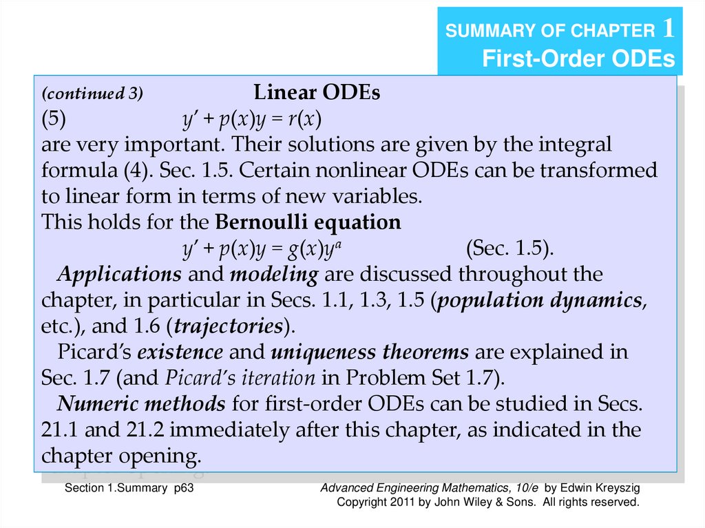
Linear ODEs
(5)
y’ + p(x)y = r(x)
are very important. Their solutions are given by the integral
formula (4). Sec. 1.5. Certain nonlinear ODEs can be transformed
to linear form in terms of new variables.
This holds for the Bernoulli equation
y’ + p(x)y = g(x)ya
(Sec. 1.5).
Applications and modeling are discussed throughout the
chapter, in particular in Secs. 1.1, 1.3, 1.5 (population dynamics,
etc.), and 1.6 (trajectories).
Picard’s existence and uniqueness theorems are explained in
Sec. 1.7 (and Picard’s iteration in Problem Set 1.7).
Numeric methods for first-order ODEs can be studied in Secs.
21.1 and 21.2 immediately after this chapter, as indicated in the
chapter opening.
(continued 3)
Section 1.Summary p63
Advanced Engineering Mathematics, 10/e by Edwin Kreyszig
Copyright 2011 by John Wiley & Sons. All rights reserved.

English Русский Правила