


 Экономика
Похожие презентации:


")

Aggregate Demand I. Building the IS–LM Model
1.
Dr.S.Sh.Sagandyko
va
Prepared by:
MACROECONOMICS
LECTURE
11
_____
Aggregate Demand I:
Building the IS–LM Model
1
2.
Outline1. 11-1 The Goods Market and the IS Curve
2. 11-2 The Money Market and the LM Curve
3. 11-3 Conclusion: The Short-Run Equilibrium
2
3. Aggregate Demand I: Building the IS–LM Model
1. Classical theory (Ch.3-7) seemed incapable of explaining theDepression.
a. national Y depends on factor supplies and the available technology,
b. neither of which changed substantially from 1929 to 1933.
c. A new model was needed.
2. In 1936 the British economist John Maynard Keynes revolutionized
economics with his book The General Theory of Employment,
Interest, and Money.
3. Keynes proposed that
a. ↓ AD is responsible for the ↓ Y & ↑ U that characterize economic ↘.
b. He criticized classical theory for assuming that AS alone determines Y.
c. Economists today reconcile these 2 views with the model of AD&AS
(Ch.10)
4. In the LR, Ps are flexible, and AS determines Y.
5. In the SR, Ps are sticky, so changes in AD influence Y.
4. Aggregate Demand I: Building the IS–LM Model
1. Our goal isa. to identify the variables that shift the AD curve, causing fls in national Y.
b. to examine the tools policymakers can use to A D .
2. (Ch. 10) We showed that monetary policy can shift the AD curve.
3. (this Ch.) We see that the government can AD with both
•. monetary and fiscal policy.
IS–LM model,
a. is the leading interpretation of Keynes’s theory.
b. The goal of the model is to show what determines national Y for a
given P.
We can view the IS–LM model as showing what causes
c. Y to change in the SR when the P is fixed because all Ps are sticky
d. the AD curve to shift.
5. Aggregate Demand I: Building the IS–LM Model
Shifts in Aggregate Demand
For a given P, national Y fluctuates because of shifts in the AD curve.
The IS–LM model takes the P as given and shows what causes Y to change.
The model therefore shows what causes AD to shift.
6.
The two parts of the IS–LM model1. the IS curve
1. stands for “investment’’ and “saving,’’
2. represents what’s going on in the market for G&S (Ch. 3).
2. The LM curve
1. stands for “liquidity’’ and “money,’’
2. Represents what’s happening to the S&D for money (Ch. 5).
The r both I & money demand, →
•. it is the variable that links the 2 halves of the IS–LM model.
3. The model shows
a. how interactions between the G & money markets determine
the position and slope of the AD curve and
b. → the level of national Y in the SR.
6
7. 11-1 The Goods Market and the IS Curve
The Keynesian CrossThe Interest Rate, Investment, and the IS Curve
How Fiscal Policy Shifs the IS Curve
11-1 The Goods Market and the IS Curve
The IS curve plots the relationship between the r & the level of Y
• that arises in the market for G&Ss.
To develop this relationship, we start with the Keynesian cross –
1. It shows how national Y is determined and
2. It is block for the IS–LM model.
In The General Theory Keynes proposed that
•. an economy’s total Y is, in the SR, determined largely by the
spending plans of H, B, and G.
> people want to spend →
> G&S firms can sell →
> Y they will choose to produce →
> workers they will choose to hire.
Keynes believed that the problem during recessions and depressions is
inadequate spending.
•. The KC is an attempt to model this insight.
8. 11-1 The Goods Market and the IS Curve
The Keynesian CrossThe Interest Rate, Investment, and the IS Curve
How Fiscal Policy Shifs the IS Curve
11-1 The Goods Market and the IS Curve
Planned Expenditure
Let us draw a distinction between actual & planned expenditure.
Actual expenditure
• is the amount Hs, Fs, & the G spend on G&S(Ch.2), it = the
economy’s GDP.
Planned expenditure
• is the amount Hs, Fs, & the G would like to spend on G&S.
Why would AE ever differ from PE?
The answer is that
• firms might engage in unplanned inventory investment because
their sales do not meet their expectations.
1. When Fs sell < of their product than they planned,
• their stock of inventories automatically r↑;
2. When Fs sell > than planned,
• their stock of inventories f↓.
These unplanned changes in inventory are counted
• as INVESTMENT spending by Fs,
• → AE can be either ͞ or _͟ PE .
9. 11-1 The Goods Market and the IS Curve
The Keynesian CrossThe Interest Rate, Investment, and the IS Curve
How Fiscal Policy Shifs the IS Curve
11-1 The Goods Market and the IS Curve
Now we consider the determinants of PE.
Assuming
• that the economy is closed, → NX = 0, →
1. PE = C + I + G. We add the consumption function:
2. C = C(Y − T)- consumption ~on disposable Y (Y − T),
• To keep things simple, we take PI as exogenously fixed:
3.
• As in Ch.3, we assume that fiscal policy— the levels of G & T—is
fixed:
4.
5.
• Combining these 5 equations, we obtain
• PE is a function of Y, the level of PI , & the fiscal policy variables.
10. Planned Expenditure as a Function of Income
PE ~ on Y because higher Y leads to ↑er consumption, which is part of PE.
The slope of the PE function is the marginal propensity to consume, MPC.
11. 11-1 The Goods Market and the IS Curve
The Keynesian CrossThe Interest Rate, Investment, and the IS Curve
How Fiscal Policy Shifs the IS Curve
11-1 The Goods Market and the IS Curve
The Economy in Equilibrium
The next assumption is that the economy is in equilibrium when AE =
PE.
• is based on the idea that
• when people’s plans have been realized, they have no reason
to change what they are doing.
Recalling that
• Y as GDP = not only total Y but also total AE on G&S, we can write
this equilibrium condition as
AE = PE
Y = PE.
The 45-degree line plots the points where this condition holds.
• With the addition of the PE function, this diagram becomes the
KC.
12.
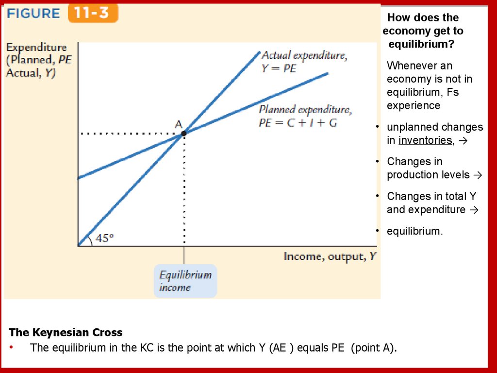
How does theeconomy get to
equilibrium?
Whenever an
economy is not in
equilibrium, Fs
experience
• unplanned changes
in inventories, →
• Changes in
production levels →
• Changes in total Y
and expenditure →
• equilibrium.
The Keynesian Cross
The equilibrium in the KC is the point at which Y (AE ) equals PE (point A).
13. The Adjustment to Equilibrium in the Keynesian Cross
• If Fs areproducing at level
Y1,
then PE1 falls short
of production, and
Fs accumulate
inventories.
• This inventory
accumulation
induces Fs to ↘
production.
Similarly, if Fs are producing at level Y2, then PE2 exceeds production, and Fs run down
their inventories.
This fall in inventories induces Fs to increase production.
In both cases, the Fs ’ decisions drive the economy toward equilibrium.
14. 11-1 The Goods Market and the IS Curve
The Keynesian CrossThe Interest Rate, Investment, and the IS Curve
How Fiscal Policy Shifs the IS Curve
11-1 The Goods Market and the IS Curve
Fiscal Policy and the Multiplier: Government Purchases
Consider how changes in G affect the economy.
• G are one component of expenditure →
• ↑er G result in ↑er PE for any given level of Y.
• If G r↗ by ∆G, then the PE schedule shifs up↑ by ∆G
• The equilibrium of the economy moves from point A to point B.
This graph shows that
• an ↗ in G → to an even greater ↗ in Y.
• → ∆Y is > ∆G.
The ratio ∆Y/∆G is called the government-purchases multiplier;
• it tells us how much I r↑ in response to a $1 ↗ in G.
• An implication of the KC is that the G multiplier is larger than 1.
15. An Increase in Government Purchases in the Keynesian Cross
Note that the ↗ in Y exceeds the ↗ in G.
→ fiscal policy has a multiplied effect on Y.
An ↗ of G
raises PE by
that amount for
any given level
of Y.
The equilibrium
moves from
point A to point
B, and Y rises
from Y1 to Y2.
16. 11-1 The Goods Market and the IS Curve
The Keynesian CrossThe Interest Rate, Investment, and the IS Curve
How Fiscal Policy Shifs the IS Curve
11-1 The Goods Market and the IS Curve
How big is the multiplier?
• we trace through each step of the change in Y.
1. Expenditure r↑ by ∆G → Y r↑ by ∆G as well.
2. This ↗ in Y in turn r↑ consumption by MPC× ∆G,
where MPC is the marginal propensity to consume.
This ↗ in consumption r↑ expenditure and Y once again.
3. This second ↗ in Y of MPC × ∆G again raises C, this time by MPC
× (MPC ×∆ G), which again ↑s expenditure and Y, and so on.
This feedback from C to Y to C continues indefinitely.
The total effect on Y is
•. Initial Change in Government Purchases = ∆G
1. First Change in Consumption = MPC × ∆G
2. Second Change in Consumption = MPC2 × ∆G
3. Third Change in Consumption = MPC3 × ∆G
4. .. .. . .
∆Y = (1 + MPC + MPC2 + MPC3 + . . .)∆G.
17. 11-1 The Goods Market and the IS Curve
The Keynesian CrossThe Interest Rate, Investment, and the IS Curve
How Fiscal Policy Shifs the IS Curve
11-1 The Goods Market and the IS Curve
The G multiplier is Y/G = 1 + MPC + MPC2 + MPC3 + . . .
This expression for the multiplier is an example of an infinite geometric
series.
A result from algebra allows us to write the multiplier as
Y/G = 1/(1 − MPC).
For example, if the MPC is 0.6, the multiplier is
Y/G = 1 + 0.6 + 0.62 + 0.63 + . . .= 1/(1 − 0.6) = 2.5.
In this case, a $1.00 increase in government purchases raises equilibrium
income by $2.50.3
18. 11-1 The Goods Market and the IS Curve
The Keynesian CrossThe Interest Rate, Investment, and the IS Curve
How Fiscal Policy Shifs the IS Curve
11-1 The Goods Market and the IS Curve
Fiscal Policy and the Multiplier: Taxes
A ↘in T of ∆T immediately r↑ disposable income Y − T by ∆T and, →
• ↗ consumption by MPC × T.
• For any given level of Y, PE is now ↑er.
• The PE schedule shifs up↑ by MPC × T.
The equilibrium of the economy moves from point A to point B.
Just as an ↗ in G has a multiplied effect on Y, → does a ↘ in Ts.
As before, the initial change in expenditure,
• now MPC × T, is multiplied by 1/(1 − MPC).
The overall effect on Y of the change in Ts is Y/T = −MPC/(1 − MPC).
This expression is the tax multiplier,
• the amount Y changes in response to a $1 change in Ts.
• The “-” sign indicates that Y moves in the opposite direction from Ts.
For example,
if the marginal propensity to consume is 0.6, then
• the tax multiplier is Y/T = −0.6/(1 − 0.6) = −1.5.
• A $1.00 cut in taxes r↑s equilibrium Y by $1.50.
19.
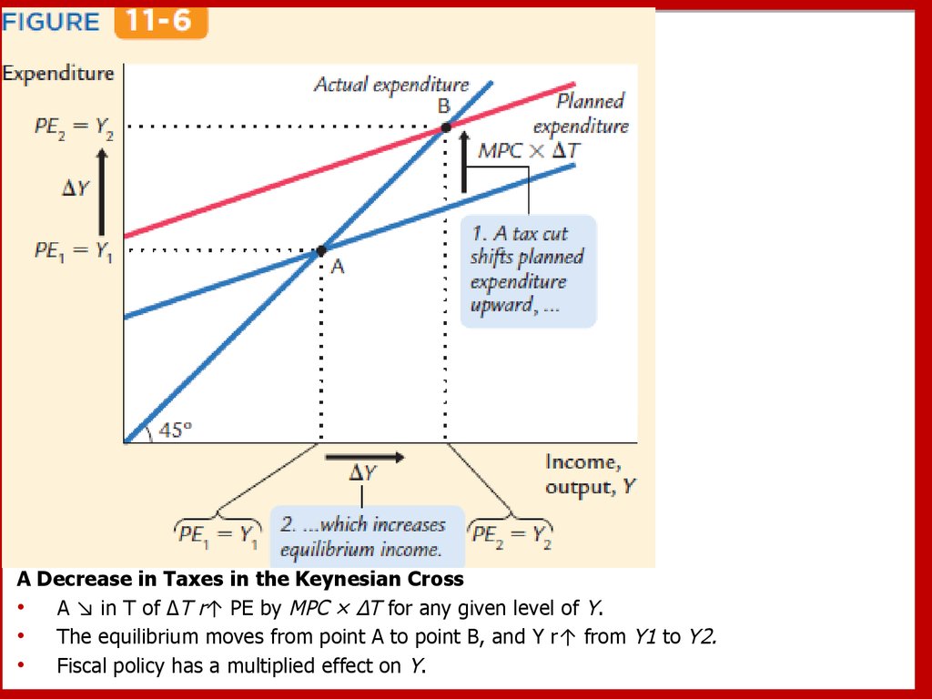
A Decrease in Taxes in the Keynesian CrossA ↘ in T of ∆T r↑ PE by MPC × ∆T for any given level of Y.
The equilibrium moves from point A to point B, and Y r↑ from Y1 to Y2.
Fiscal policy has a multiplied effect on Y.
20. Cutting Taxes to Stimulate the Economy: The Kennedy and Bush Tax Cuts
CaseStudy
John F. Kennedy became president of the United States in 1961.
• One of the council’s first proposals was to expand national Y by reducing
taxes.
• Tax cuts stimulate aggregate supply by improving workers’ incentives and
expand AD by raising households’ disposable Y.
• GDP ↗, U ↘
George W. Bush was elected president in 2000, a major element of his platform
was a cut in Y taxes.
• Bush used both supply-side and Keynesian rhetoric to make the case for their
policy.
• When people have more M., they can spend it on G&S.
• When they demand an additional G&S, somebody will produce the G or S.
• When somebody produces that G&S, it means somebody is more likely to be
able to find a job.
• GDP ↗, U ↘
21. Increasing Government Purchases to Stimulate the Economy: The Obama Spending Plan
CaseStudy
When President Barack Obama took office in January 2009, the economy was
suffering from a significant recession.
• The package included some tax cuts and higher transfer payments, but much
of it was made up of ↗ in G of G&S.
Congress went ahead with President Obama’s proposed stimulus plans with
relatively minor modifications.
• The president signed the $787 billion billon February 17, 2009.
Did it work?
• The economy did recover from the recession,
• but much more slowly than the Obama administration economists initially
forecast.
Whether the slow recovery reflects
1. the failure of stimulus policy or
2. a sicker economy than the economists first appreciated
is a question of continuing debate.
22. 11-1 The Goods Market and the IS Curve
The Keynesian CrossThe Interest Rate, Investment, and the IS Curve
How Fiscal Policy Shifs the IS Curve
11-1 The Goods Market and the IS Curve
The KС
• explains the economy’s AD curve
• shows how the spending plans of H, F, the G determine the Y.
• makes the assumption that the level of PI is fixed.
An important macroeconomic relationship is that PI ~ on the r (Ch.3).
To add this relationship between the r & I to our model,
• we write the level of PI as I = I(r).
The r is the cost of borrowing to finance investment projects
→ an ↗ in the r reduces PI.
→ the investment function slopes downward.
To determine how Y changes when the r changes,
• we can combine the investment function with the KС diagram.
23.
Deriving the IS CurvePanel (a) shows the investment function:
an ↗ in the r from r1 to r2 reduces PI from
I(r1) to I(r2).
Panel (b) shows the KC:
a ↘ in PI from I(r1) to I(r2) shifts the PE
function ↘ and → reduces Y from Y1 to Y2.
Panel (c) shows the IS curve summarizing
this relationship between the r and Y:
the ↑er the r, the ↓er the level of Y.
24. 11-1 The Goods Market and the IS Curve
The Keynesian CrossThe Interest Rate, Investment, and the IS Curve
How Fiscal Policy Shifs the IS Curve
11-1 The Goods Market and the IS Curve
The IS curve shows us,
• for any given r, the level of Y that brings the goods market into
equilibrium.
As we learned from the KC,
• the equilibrium level of Y also ~on Gnt spending G and taxes T.
The IS curve is drawn for a given FP; that is,
• when we construct the IS curve, we hold G and T fixed.
• When FP changes, the IS curve shifs.
Changes in FP that
1. r↑ the demand for G&S shif the IS curve to the right.
2. r↓ the demand for G&S shif the IS curve to the left.
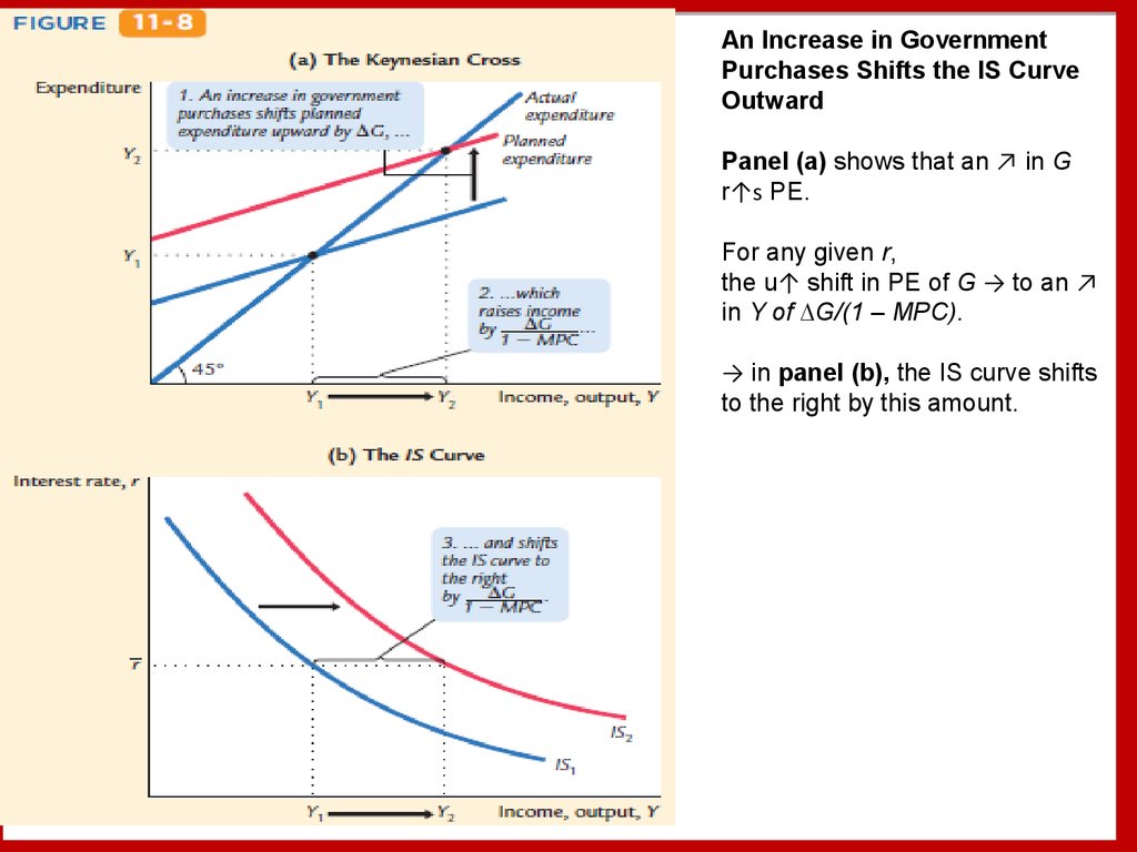
25.
An Increase in GovernmentPurchases Shifts the IS Curve
Outward
Panel (a) shows that an ↗ in G
r↑s PE.
For any given r,
the u↑ shift in PE of G → to an ↗
in Y of ∆G/(1 – MPC).
→ in panel (b), the IS curve shifts
to the right by this amount.
26. 11-2 The Money Market and the LM Curve
The Theory of Liquidity PreferenceIncome, Money Demand, and the LM Curve
How Monetary Policy Shifs the LM Curve
11-2 The Money Market and the LM Curve
27. The Theory of Liquidity Preference
The S&D for RMB determing the r.
The S curve for RMB is vertical because the S does not ~on the r.
The D curve is d↓ sloping because a ↑er r
1. r↑ the cost of holding money and →
2. lowers the quantity demanded.
At the equilibrium r, the quantity of RMB demanded = the quantity supplied.
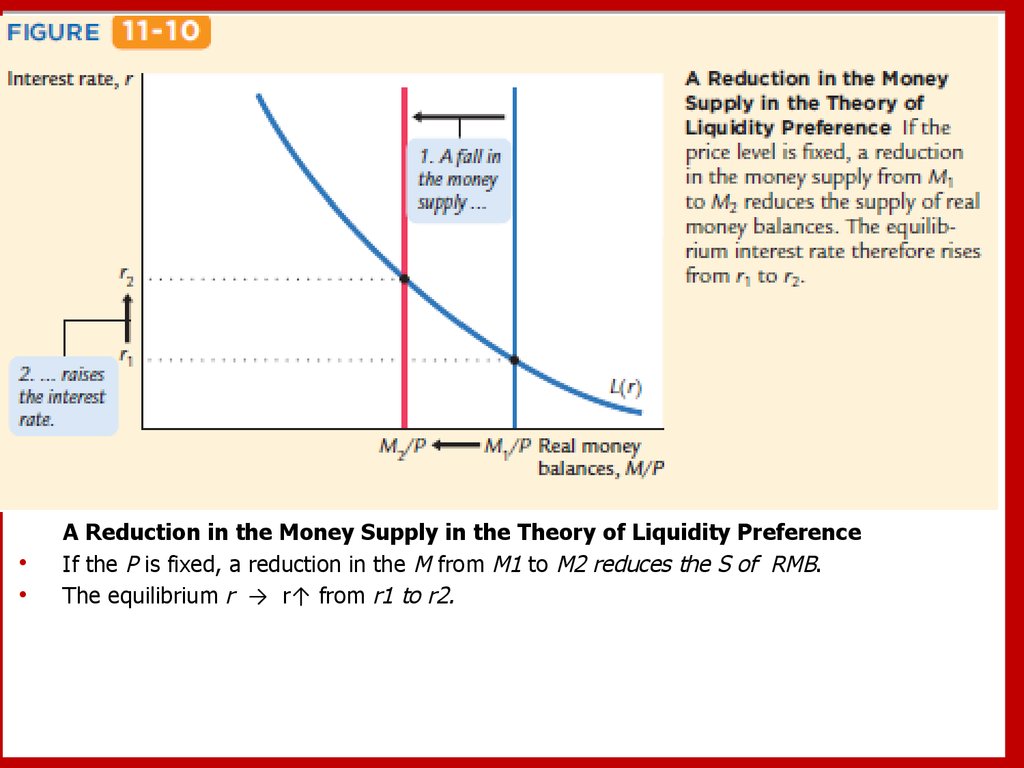
28.
A Reduction in the Money Supply in the Theory of Liquidity Preference
If the P is fixed, a reduction in the M from M1 to M2 reduces the S of RMB.
The equilibrium r → r↑ from r1 to r2.
29. Does a Monetary Tightening Raise or Lower Interest Rates?
CaseStudy
Does a Monetary Tightening Raise or Lower Interest Rates?
30. 11-2 The Money Market and the LM Curve
The Theory of Liquidity PreferenceIncome, Money Demand, and the LM Curve
How Monetary Policy Shifs the LM Curve
11-2 The Money Market and the LM Curve
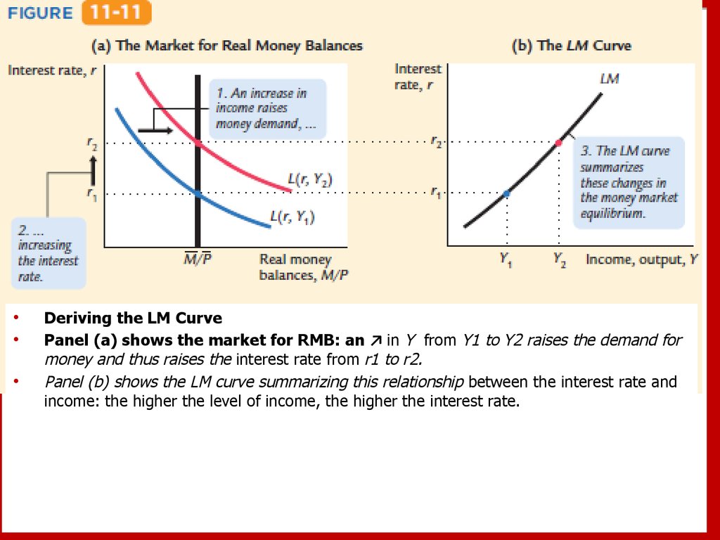
31.
Deriving the LM Curve
Panel (a) shows the market for RMB: an ↗ in Y from Y1 to Y2 raises the demand for
money and thus raises the interest rate from r1 to r2.
Panel (b) shows the LM curve summarizing this relationship between the interest rate and
income: the higher the level of income, the higher the interest rate.
32. 11-2 The Money Market and the LM Curve
The Theory of Liquidity PreferenceIncome, Money Demand, and the LM Curve
How Monetary Policy Shifs the LM Curve
11-2 The Money Market and the LM Curve
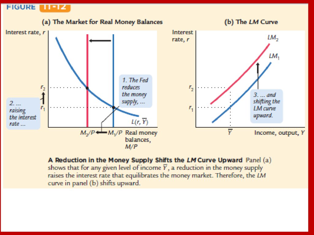
The LM curve shows the combinations of the interest rate and the
level of Y that are consistent with equilibrium in the market for RMB.
The LM curve is drawn for a given supply of RMB.
• ↘ in the supply of RMB shift the LM curve u↑.
• ↗in the supply of RMB shift the LM curve d↓.
33.
34. 11-3 Conclusion: The Short-Run Equilibrium
We now have all the pieces of the IS–LM model.The two equations of this model are
1. Y = C(Y − T ) + I(r) + G - IS,
2. M/P = L(r, Y)
- LM.
35.
Equilibrium in the
IS–LM Model
The intersection of the IS and LM curves represents simultaneous equilibrium
in the market for G&S & in the market for RMB
for given values of Gnt spending, T, the M, and the P.
36.
The Theory of Short-Run FluctuationsThis schematic diagram shows how the different pieces of the theory of SR fluctuations fit
together.
1. The KC explains the IS curve, and the TLP explains the LM curve.
2. The IS and LM curves together yield the IS–LM model, which explains the AD curve.
3. The AD curve is part of the model of AS & AD, which economists use to explain SR
fluctuations in economic activity.