


 Математика
 Менеджмент
Похожие презентации:


. Week 8")


Linear Regression and Correlation Analysis
1.
Chapter 14Introduction to Linear
Regression and
Correlation Analysis
ALWAYS LEARNING
Copyright © 2018 Pearson Education, Ltd.
Slide - 1
2.
Learning OutcomesOutcome 1. Calculate and interpret the correlation between two variables.
Outcome 2. Determine whether the correlation is significant.
Outcome 3. Calculate the simple linear regression equation for a set of data and
know the basic assumptions behind regression analysis
Outcome 4. Determine whether a regression model is significant.
Outcome 5. Recognize regression analysis applications for purposes of
description and prediction.
Outcome 6. Calculate and interpret confidence intervals for the regression analysis.
Outcome 7. Recognize some potential problems if regression analysis is used
incorrectly.
ALWAYS LEARNING
Copyright © 2018 Pearson Education, Ltd.
Slide - 2
3.
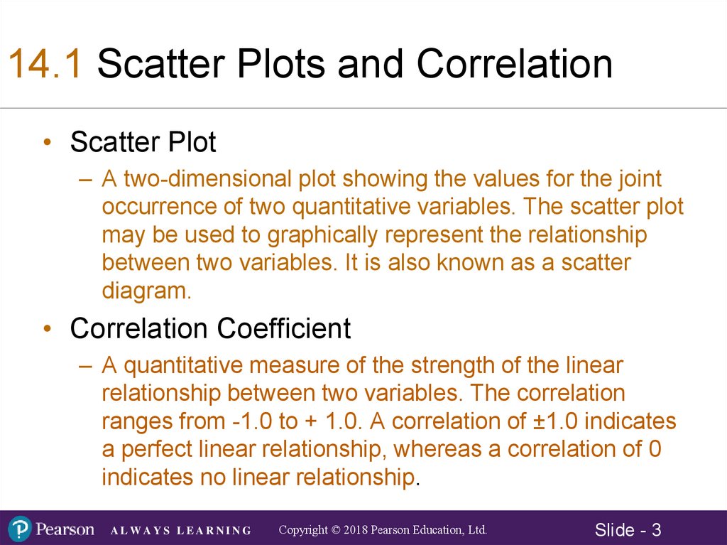
14.1 Scatter Plots and Correlation• Scatter Plot
– A two-dimensional plot showing the values for the joint
occurrence of two quantitative variables. The scatter plot
may be used to graphically represent the relationship
between two variables. It is also known as a scatter
diagram.
• Correlation Coefficient
– A quantitative measure of the strength of the linear
relationship between two variables. The correlation
ranges from -1.0 to + 1.0. A correlation of ±1.0 indicates
a perfect linear relationship, whereas a correlation of 0
indicates no linear relationship.
ALWAYS LEARNING
Copyright © 2018 Pearson Education, Ltd.
Slide - 3
4.
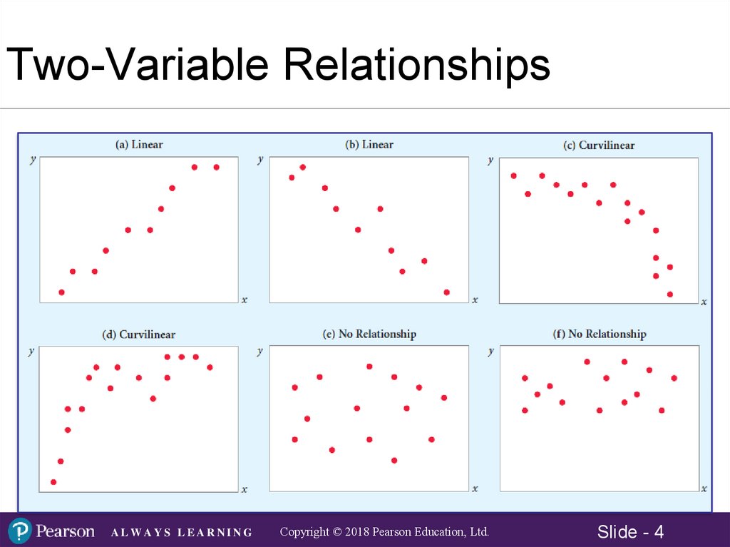
Two-Variable RelationshipsALWAYS LEARNING
Copyright © 2018 Pearson Education, Ltd.
Slide - 4
5.
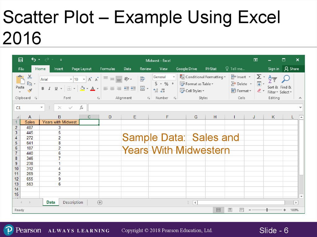
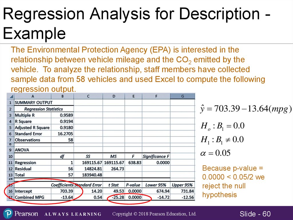
Scatter Plot – Example Using Excel2016
The director of marketing for Midwest Distribution
Company is concerned about the rapid turnover in
her sales force. In the course of exit interviews,
she discovered a major concern with the
compensation structure. At issue is the
relationship between sales and number of years
with the company. The data for a random sample
of 12 sales representatives was used for analysis.
Objective: Use Excel 2016 to first create a scatter
plot using the data file Midwest.xlsx.
ALWAYS LEARNING
Copyright © 2018 Pearson Education, Ltd.
Slide - 5
6.
Scatter Plot – Example Using Excel2016
Sample Data: Sales and
Years With Midwestern
ALWAYS LEARNING
Copyright © 2018 Pearson Education, Ltd.
Slide - 6
7.
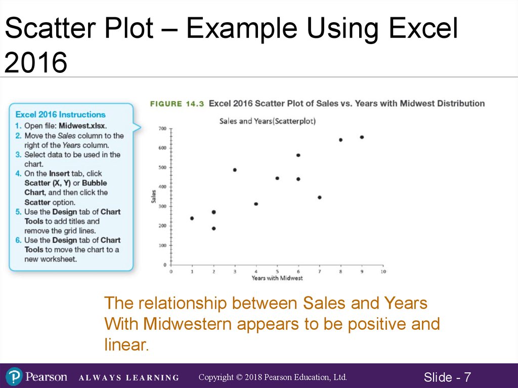
Scatter Plot – Example Using Excel2016
The relationship between Sales and Years
With Midwestern appears to be positive and
linear.
ALWAYS LEARNING
Copyright © 2018 Pearson Education, Ltd.
Slide - 7
8.
The Correlation Coefficient• Sample Correlation Coefficient:
• Algebraic Equivalent:
r - Sample correlation coefficient
n - Sample size
x - Value of the independent variable
y - Value of the dependent variable
ALWAYS LEARNING
Copyright © 2018 Pearson Education, Ltd.
Slide - 8
9.
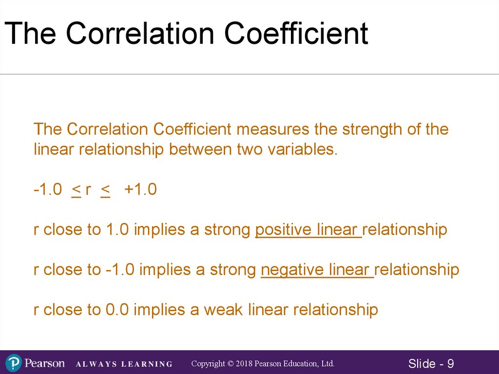
The Correlation CoefficientThe Correlation Coefficient measures the strength of the
linear relationship between two variables.
-1.0 < r < +1.0
r close to 1.0 implies a strong positive linear relationship
r close to -1.0 implies a strong negative linear relationship
r close to 0.0 implies a weak linear relationship
ALWAYS LEARNING
Copyright © 2018 Pearson Education, Ltd.
Slide - 9
10.
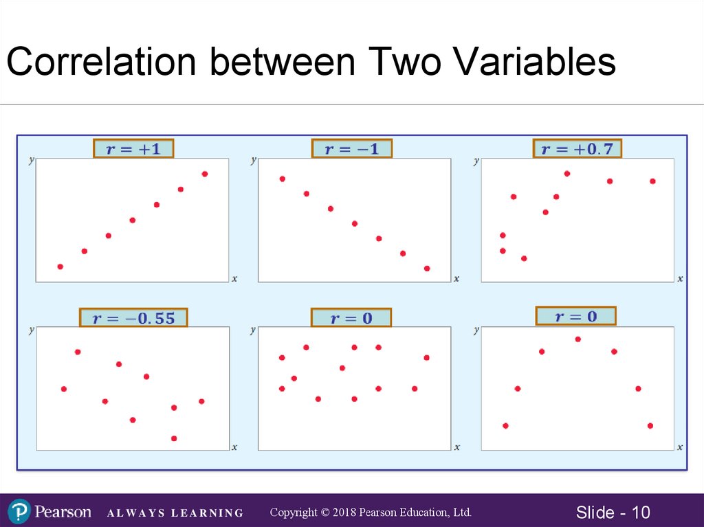
Correlation between Two VariablesALWAYS LEARNING
Copyright © 2018 Pearson Education, Ltd.
Slide - 10
11.
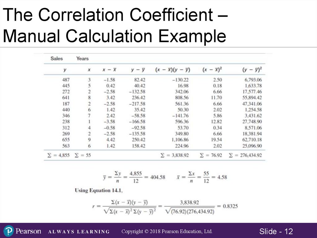
The Correlation Coefficient ExampleThe company is studying the relationship between sales (on which
commissions are paid) and number of years a sales person is with the
company. A random sample of 12 sales representatives is collected.
Compute the correlation coefficient.
700
600
Sales
500
400
300
200
100
1
2
3
4
5
6
7
8
9
10
Years
ALWAYS LEARNING
Copyright © 2018 Pearson Education, Ltd.
Slide - 11
12.
The Correlation Coefficient –Manual Calculation Example
ALWAYS LEARNING
Copyright © 2018 Pearson Education, Ltd.
Slide - 12
13.
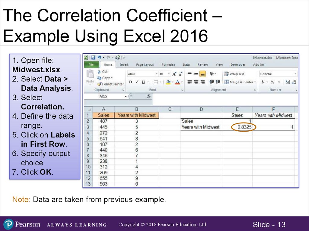
The Correlation Coefficient –Example Using Excel 2016
1. Open file:
Midwest.xlsx.
2. Select Data >
Data Analysis.
3. Select
Correlation.
4. Define the data
range.
5. Click on Labels
in First Row.
6. Specify output
choice.
7. Click OK.
Note: Data are taken from previous example.
ALWAYS LEARNING
Copyright © 2018 Pearson Education, Ltd.
Slide - 13
14.
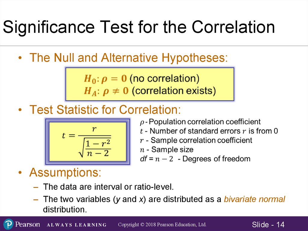
Significance Test for the Correlation• The Null and Alternative Hypotheses:
• Test Statistic for Correlation:
• Assumptions:
– The data are interval or ratio-level.
– The two variables (y and x) are distributed as a bivariate normal
distribution.
ALWAYS LEARNING
Copyright © 2018 Pearson Education, Ltd.
Slide - 14
15.
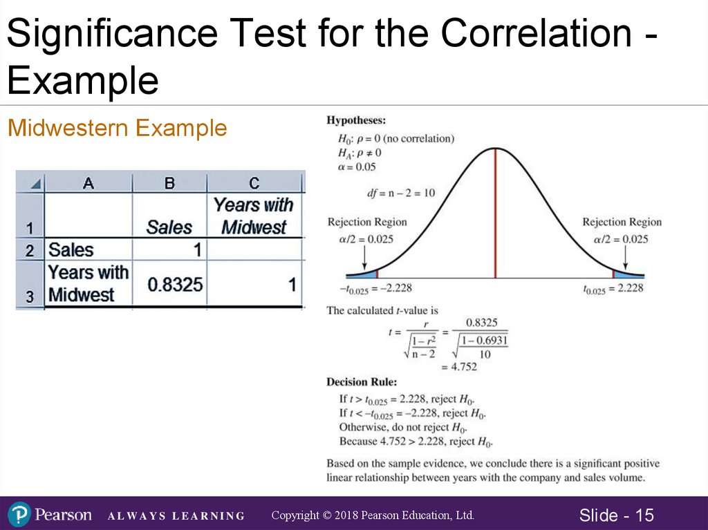
Significance Test for the Correlation ExampleMidwestern Example
ALWAYS LEARNING
Copyright © 2018 Pearson Education, Ltd.
Slide - 15
16.
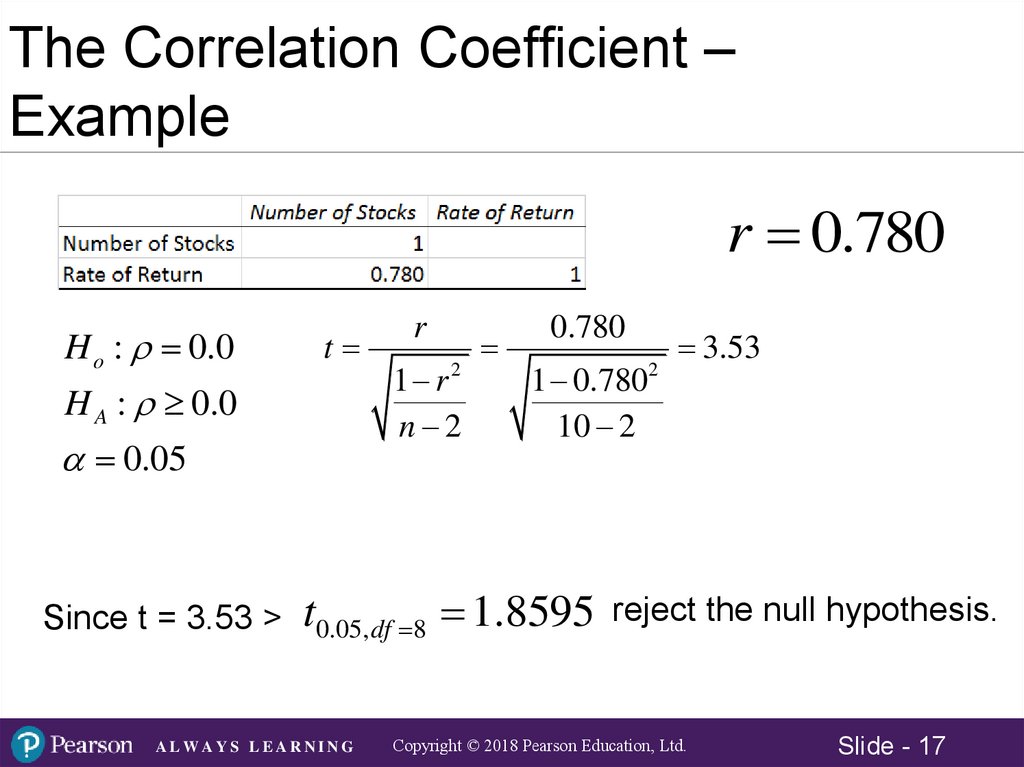
The Correlation Coefficient –Example
A money management company is interested in
determining whether there is a positive linear
relationship between the number of stocks in a
client’s portfolio and the portfolio annual rate of
return. A sample of n=10 clients has been
selected. The sample data are:
ALWAYS LEARNING
Copyright © 2018 Pearson Education, Ltd.
Slide - 16
17.
The Correlation Coefficient –Example
r 0.780
H o : 0.0
t
H A : 0.0
0.05
Since t = 3.53 >
r
1 r
n 2
2
0.780
1 0.780
10 2
t0.05,df 8 1.8595
ALWAYS LEARNING
2
3.53
reject the null hypothesis.
Copyright © 2018 Pearson Education, Ltd.
Slide - 17
18.
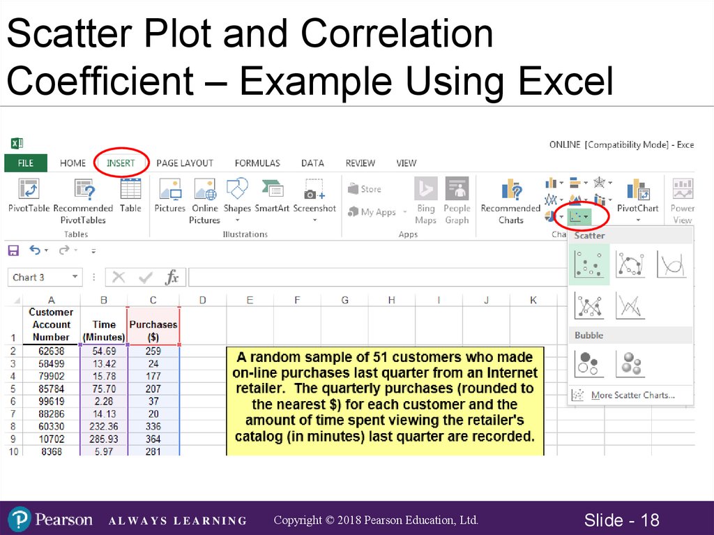
Scatter Plot and CorrelationCoefficient – Example Using Excel
ALWAYS LEARNING
Copyright © 2018 Pearson Education, Ltd.
Slide - 18
19.
Scatter Plot and CorrelationCoefficient – Example Using Excel
ALWAYS LEARNING
Copyright © 2018 Pearson Education, Ltd.
Slide - 19
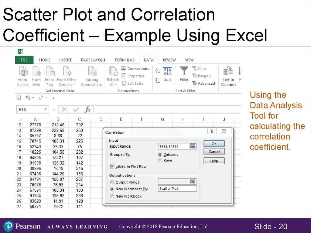
20.
Scatter Plot and CorrelationCoefficient – Example Using Excel
Using the
Data Analysis
Tool for
calculating the
correlation
coefficient.
ALWAYS LEARNING
Copyright © 2018 Pearson Education, Ltd.
Slide - 20
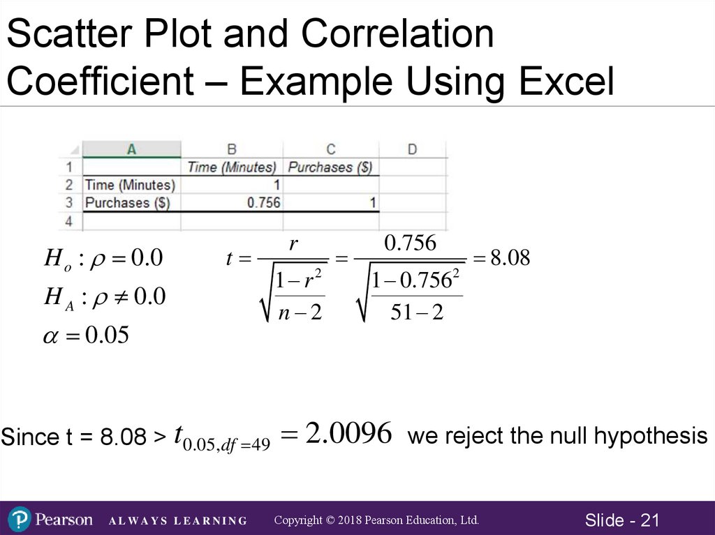
21.
Scatter Plot and CorrelationCoefficient – Example Using Excel
H o : 0.0
t
H A : 0.0
0.05
Since t = 8.08 > t0.05, df 49
ALWAYS LEARNING
r
1 r
n 2
2
0.756
1 0.756
51 2
2.0096
2
8.08
we reject the null hypothesis
Copyright © 2018 Pearson Education, Ltd.
Slide - 21
22.
Correlation Analysis - Summary• Step 1: Specify the population parameter of interest
• Step 2: Formulate the appropriate null and
alternative hypotheses
• Step 3: Specify the level of significance
• Step 4: Compute the correlation coefficient and the
test statistic
• Step 5: Construct the rejection region and decision
rule.
• Step 6: Reach a decision
• Step 7: Draw a conclusion
ALWAYS LEARNING
Copyright © 2018 Pearson Education, Ltd.
Slide - 22
23.
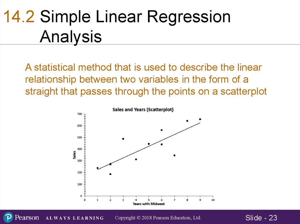
14.2 Simple Linear RegressionAnalysis
A statistical method that is used to describe the linear
relationship between two variables in the form of a
straight that passes through the points on a scatterplot
ALWAYS LEARNING
Copyright © 2018 Pearson Education, Ltd.
Slide - 23
24.
Simple Linear Regression Analysis• When there are only two variables - a dependent
variable, and an independent variable, the
technique is referred to as simple regression
analysis
• When the relationship between the dependent
variable and the independent variable is linear,
the technique is simple linear regression
ALWAYS LEARNING
Copyright © 2018 Pearson Education, Ltd.
Slide - 24
25.
Dependent and IndependentVariables
Dependent Variable – A variable whose values are
thought to be a function of, or dependent on, the values of
more or more other variables. This dependent variable is
referred to as the y variable and is placed on the vertical
axis of a scatterplot.
The Independent Variable – A variable whose values are
thought to influence the values of the dependent variable.
Independent variables are also called explanatory
variables. The dependent variable is referred to as the x
variable and is placed on the horizontal axis of a
scatterplot.
ALWAYS LEARNING
Copyright © 2018 Pearson Education, Ltd.
Slide - 25
26.
The Regression ModelALWAYS LEARNING
Copyright © 2018 Pearson Education, Ltd.
Slide - 26
27.
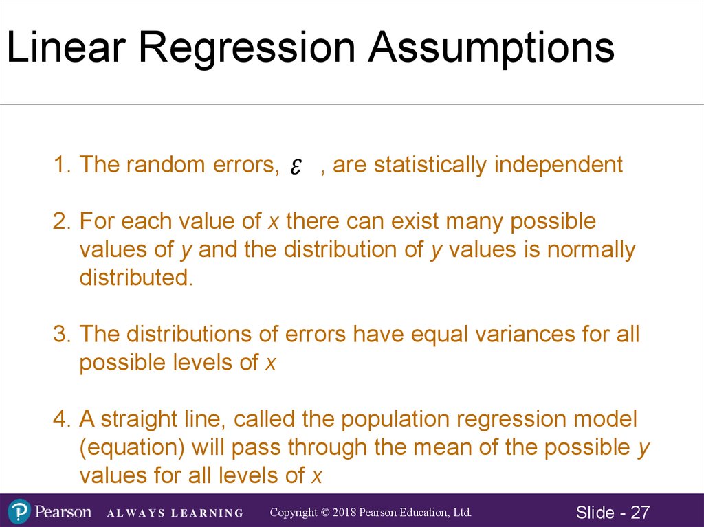
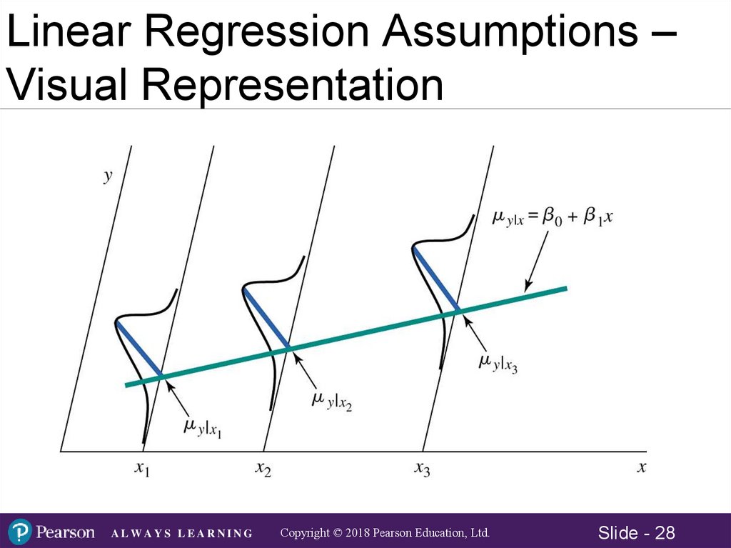
Linear Regression Assumptions1. The random errors,
, are statistically independent
2. For each value of x there can exist many possible
values of y and the distribution of y values is normally
distributed.
3. The distributions of errors have equal variances for all
possible levels of x
4. A straight line, called the population regression model
(equation) will pass through the mean of the possible y
values for all levels of x
ALWAYS LEARNING
Copyright © 2018 Pearson Education, Ltd.
Slide - 27
28.
Linear Regression Assumptions –Visual Representation
ALWAYS LEARNING
Copyright © 2018 Pearson Education, Ltd.
Slide - 28
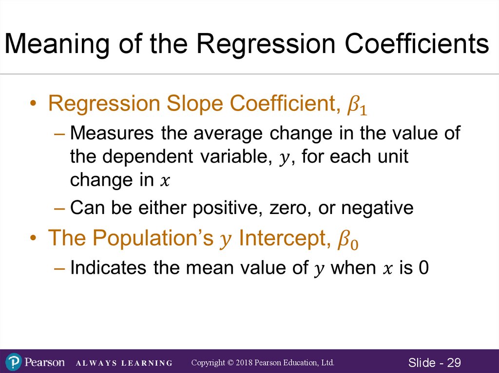
29.
Meaning of the Regression CoefficientsALWAYS LEARNING
Copyright © 2018 Pearson Education, Ltd.
Slide - 29
30.
Estimates of the RegressionCoefficients
yˆ bo b1 x
where :
yˆ estimated value of the dependent variable for a given value of x
b1 estimate of the true population regression slope coefficient
bo estimate of the true population y intercept
How do we determine the values for bo and b1 ?
ALWAYS LEARNING
Copyright © 2018 Pearson Education, Ltd.
Slide - 30
31.
Regression Line ExamplesWhich Regression Line is Best? Examine Regression Errors
ALWAYS LEARNING
Copyright © 2018 Pearson Education, Ltd.
Slide - 31
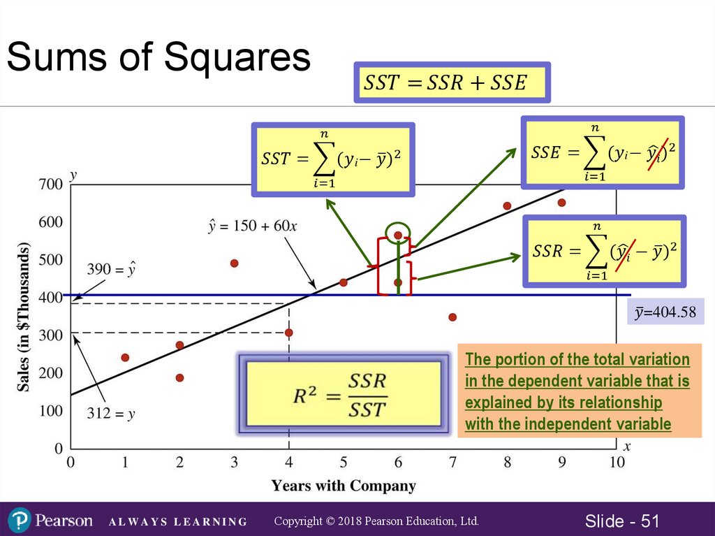
32.
Computation of Regression Error Examplen
min ( yi yˆ ) 2
i 1
ALWAYS LEARNING
Copyright © 2018 Pearson Education, Ltd.
Slide - 32
33.
Least Squares Criterion• The criterion for determining a regression
line that minimizes the sum of squared
prediction errors (residuals)
n
min ( yi yˆ ) 2
Sum of Squared Residual (Errors) = SSE
i 1
Residual
• Residual: The difference between the
actual value of the dependent variable and
the value predicted by the regression
model.
ALWAYS LEARNING
Copyright © 2018 Pearson Education, Ltd.
Slide - 33
34.
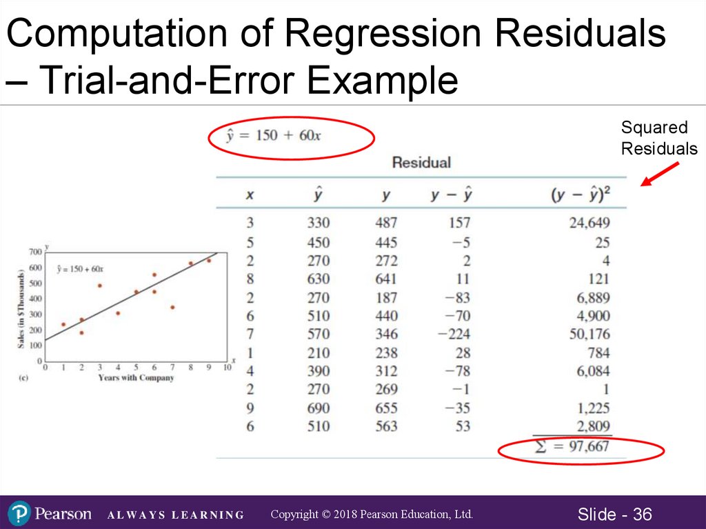
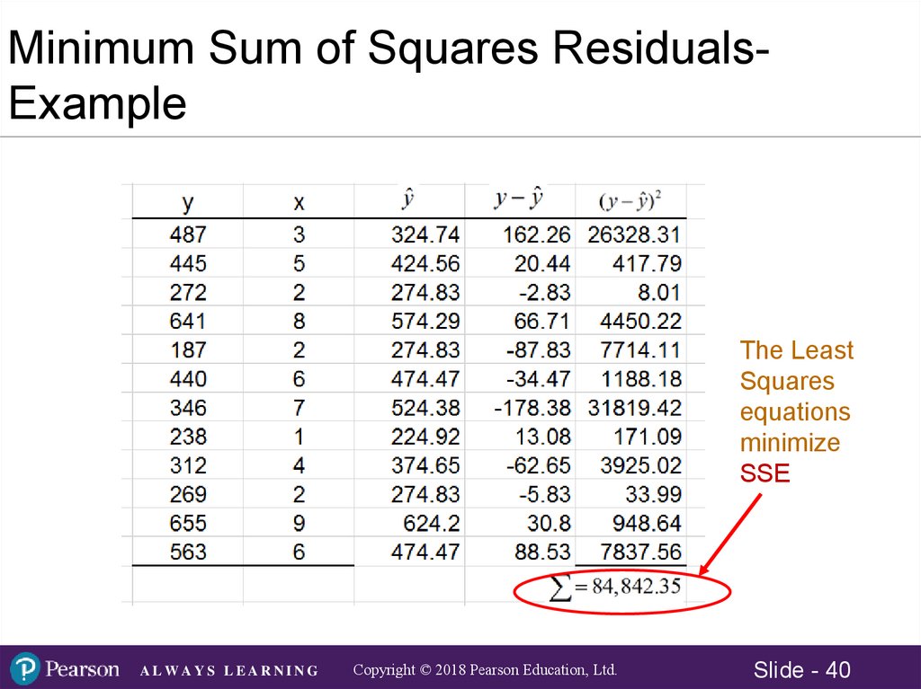
Computation of Regression Residuals– Trial-and-Error Example
Squared
Residuals
Sum of Squared Residuals (Errors) =
ALWAYS LEARNING
Copyright © 2018 Pearson Education, Ltd.
Slide - 34
35.
Computation of Regression Residuals– Trial-and-Error Example
Squared
Residuals
ALWAYS LEARNING
Copyright © 2018 Pearson Education, Ltd.
Slide - 35
36.
Computation of Regression Residuals– Trial-and-Error Example
Squared
Residuals
ALWAYS LEARNING
Copyright © 2018 Pearson Education, Ltd.
Slide - 36
37.
Least Squares CriterionWe need a more direct approach than trial-and-error! The
answer lies in finding the slope and intercept such that the
sum of squared residuals is minimized for the sample data.
n
Sum of Squared
Residuals (Errors)
= SSE
2
ˆ
min ( yi y )
i 1
The least squares equations:
n
b1
( xi x )( yi y )
i 1
n
2
(
x
x
)
i
and
bo y b1 x
i 1
ALWAYS LEARNING
Copyright © 2018 Pearson Education, Ltd.
Slide - 37
38.
Least Squares Equations – ManualCalculations Example
n
b1
( x x )( y y )
i 1
n
(x x )
2
3838.92
49.91
76.92
bo y b1 x = 404.6 (49.91)(4.6) 175.01
i 1
ALWAYS LEARNING
Copyright © 2018 Pearson Education, Ltd.
Slide - 38
39.
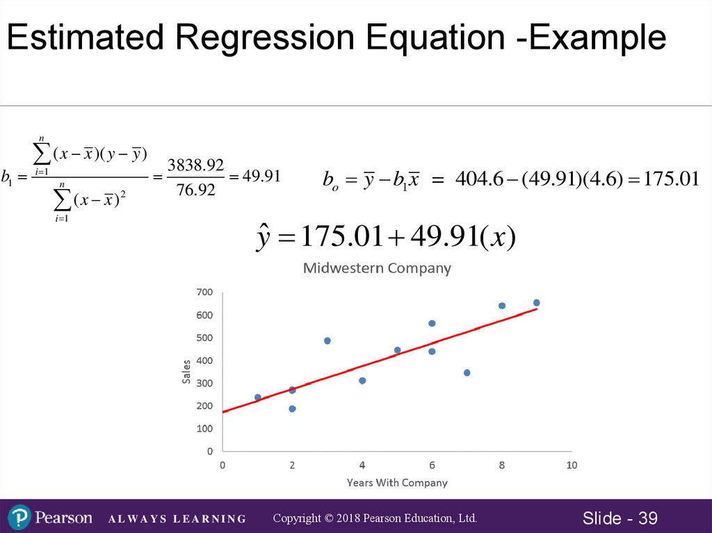
Estimated Regression Equation -Examplen
b1
( x x )( y y )
i 1
n
(x x )
2
3838.92
49.91
76.92
i 1
bo y b1 x = 404.6 (49.91)(4.6) 175.01
yˆ 175.01 49.91( x)
ALWAYS LEARNING
Copyright © 2018 Pearson Education, Ltd.
Slide - 39
40.
Minimum Sum of Squares ResidualsExampleThe Least
Squares
equations
minimize
SSE
ALWAYS LEARNING
Copyright © 2018 Pearson Education, Ltd.
Slide - 40
41.
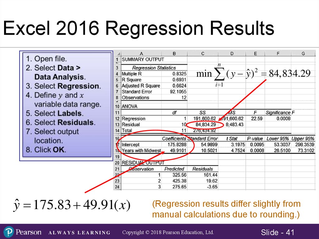
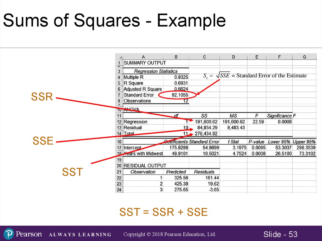
Excel 2016 Regression Resultsn
min ( y yˆ ) 2 84,834.29
i 1
yˆ 175.83 49.91( x)
ALWAYS LEARNING
(Regression results differ slightly from
manual calculations due to rounding.)
Copyright © 2018 Pearson Education, Ltd.
Slide - 41
42.
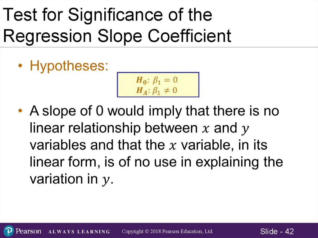
Test for Significance of theRegression Slope Coefficient
ALWAYS LEARNING
Copyright © 2018 Pearson Education, Ltd.
Slide - 42
43.
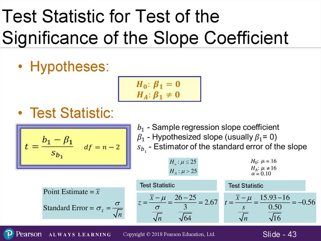
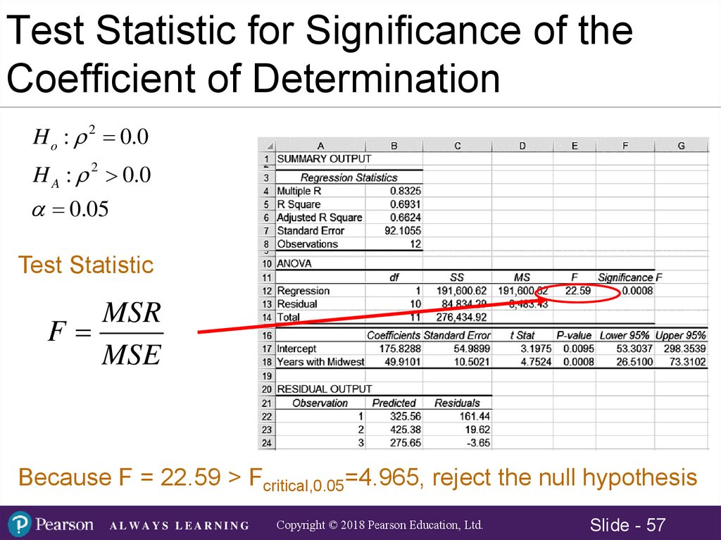
Test Statistic for Test of theSignificance of the Slope Coefficient
• Hypotheses:
• Test Statistic:
H o : 25
H A : 25
Test Statistic
Point Estimate = x
Standard Error = x
ALWAYS LEARNING
n
z
x
n
Test Statistic
26 25
x 15.93 16
2.67 t
0.56
3
s
0.50
64
n
16
Copyright © 2018 Pearson Education, Ltd.
Slide - 43
44.
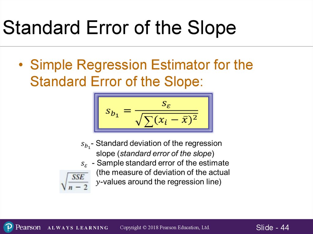
Standard Error of the Slope• Simple Regression Estimator for the
Standard Error of the Slope:
ALWAYS LEARNING
Copyright © 2018 Pearson Education, Ltd.
Slide - 44
45.
Standard Error of the SlopeLarge Standard Error
ALWAYS LEARNING
Small Standard Error
Copyright © 2018 Pearson Education, Ltd.
Slide - 45
46.
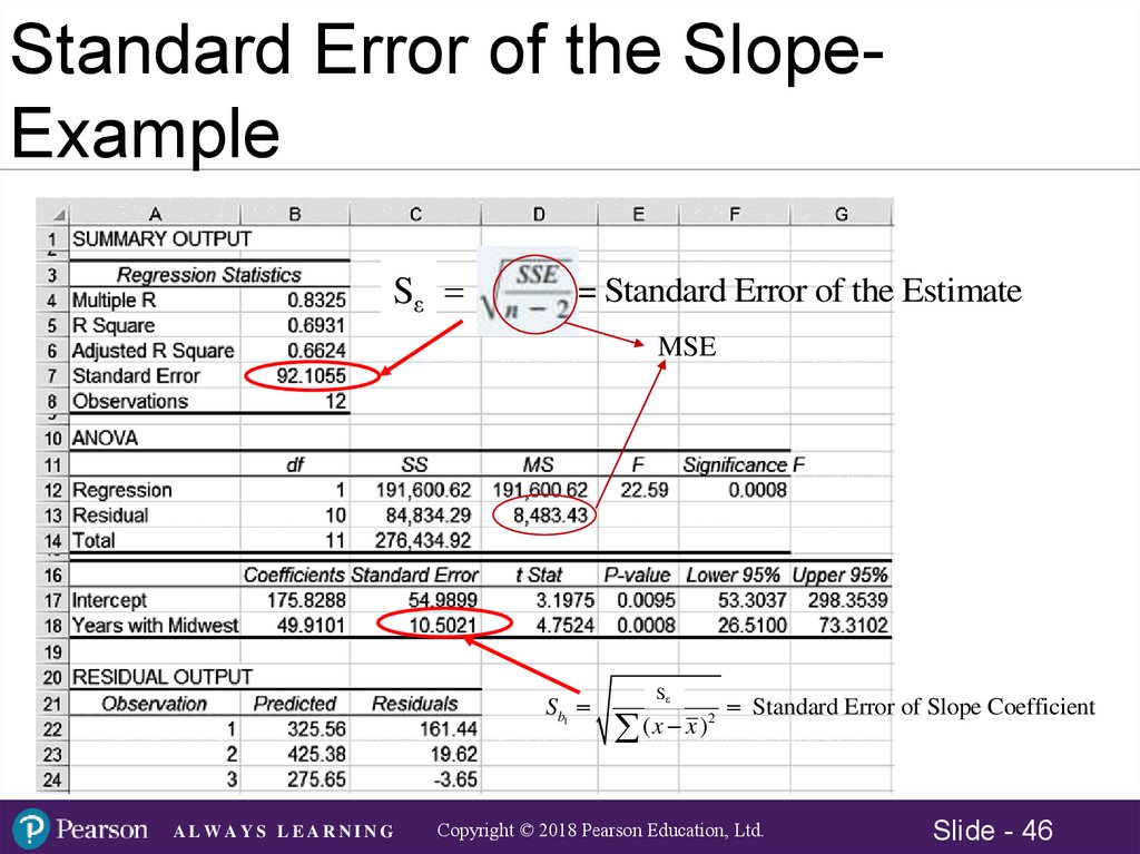
Standard Error of the SlopeExampleSSεe
SSE = Standard Error of the Estimate
MSE
Sb1
ALWAYS LEARNING
SSεe
Standard Error of Slope Coefficient
2
(
x
x
)
Copyright © 2018 Pearson Education, Ltd.
Slide - 46
47.
Test Statistic for Test of theSignificance of the Slope Coefficient
H o : B1 0.0
H1 : B1 0.0
0.05
Test Statistic
t
b1 B1 49.91 0.0
4.752
Sb1
10.5021
ALWAYS LEARNING
Copyright © 2018 Pearson Education, Ltd.
Slide - 47
48.
Test Statistic for Test of theSignificance of the Slope Coefficient
ALWAYS LEARNING
Copyright © 2018 Pearson Education, Ltd.
Slide - 48
49.
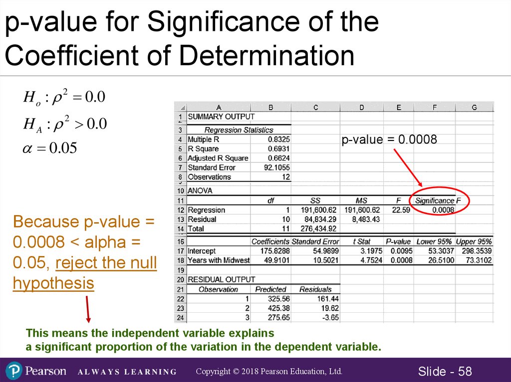
p-value for Test of theSignificance of the Slope Coefficient
H o : B1 0.0
H1 : B1 0.0
0.05
p-value
Because p-value = 0.0008 < alpha/2 = 0.025, reject Ho
ALWAYS LEARNING
Copyright © 2018 Pearson Education, Ltd.
Slide - 49
50.
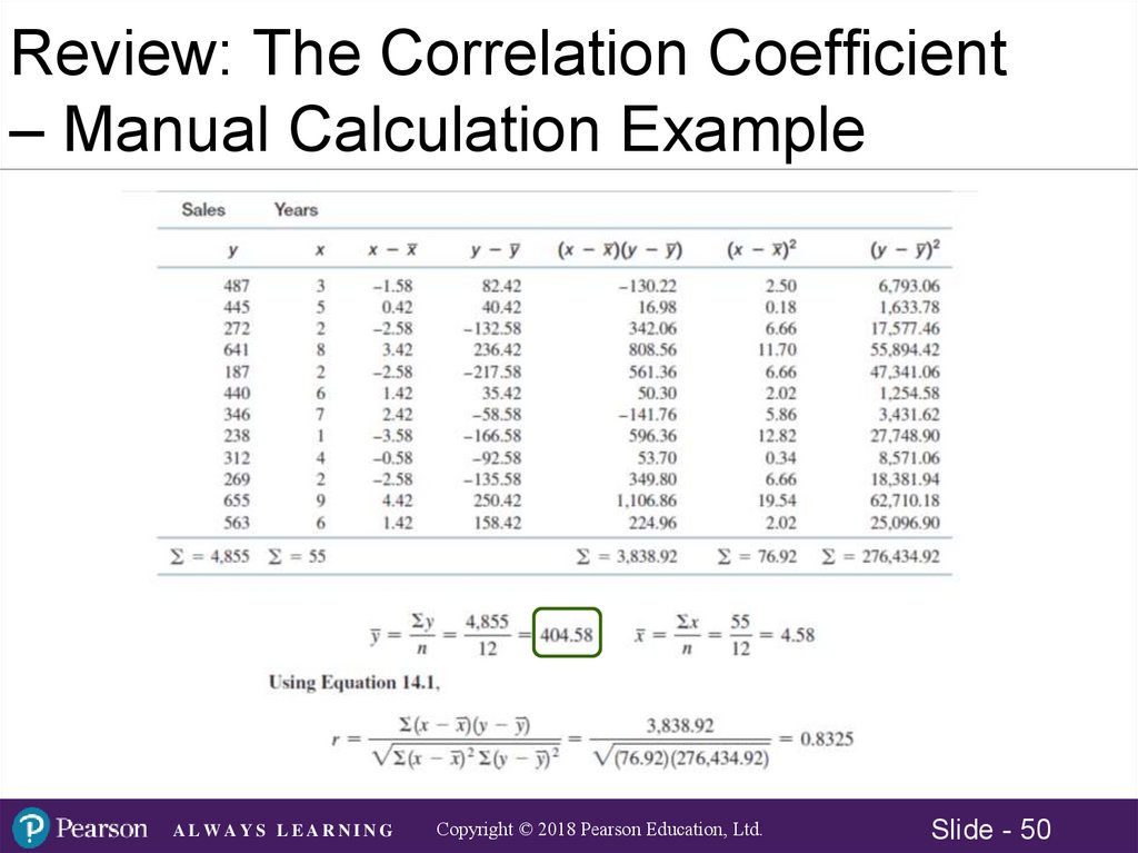
Review: The Correlation Coefficient– Manual Calculation Example
ALWAYS LEARNING
Copyright © 2018 Pearson Education, Ltd.
Slide - 50