


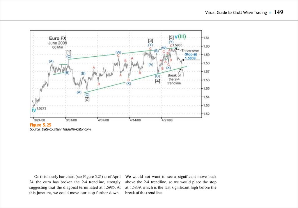
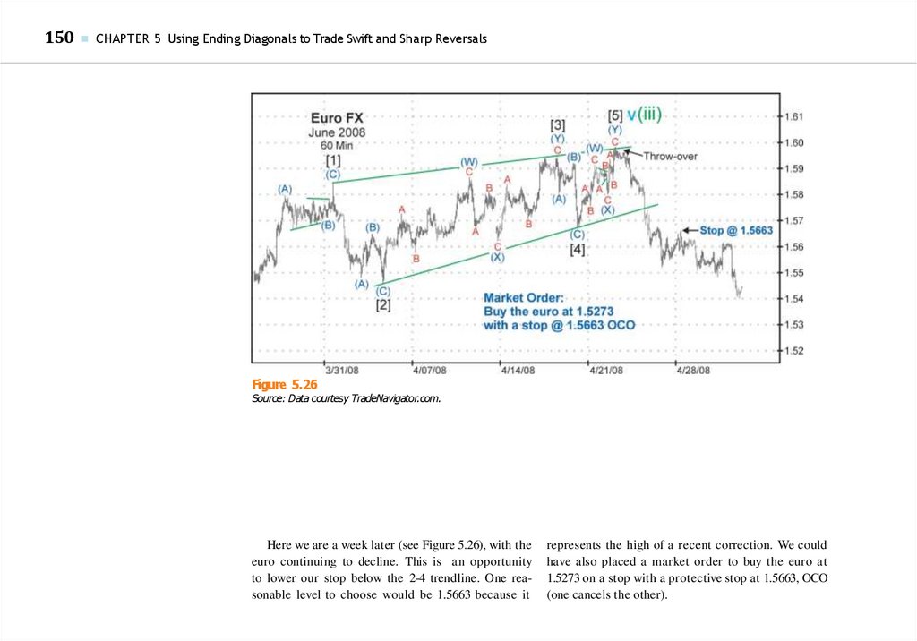
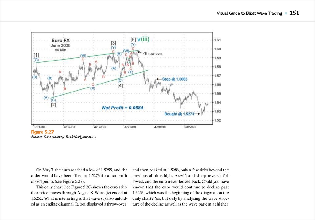


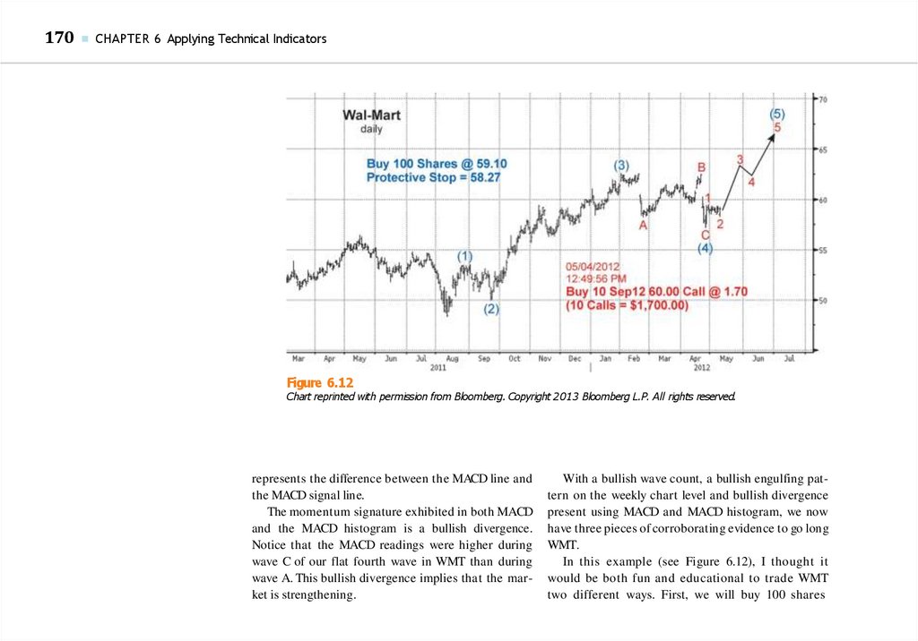
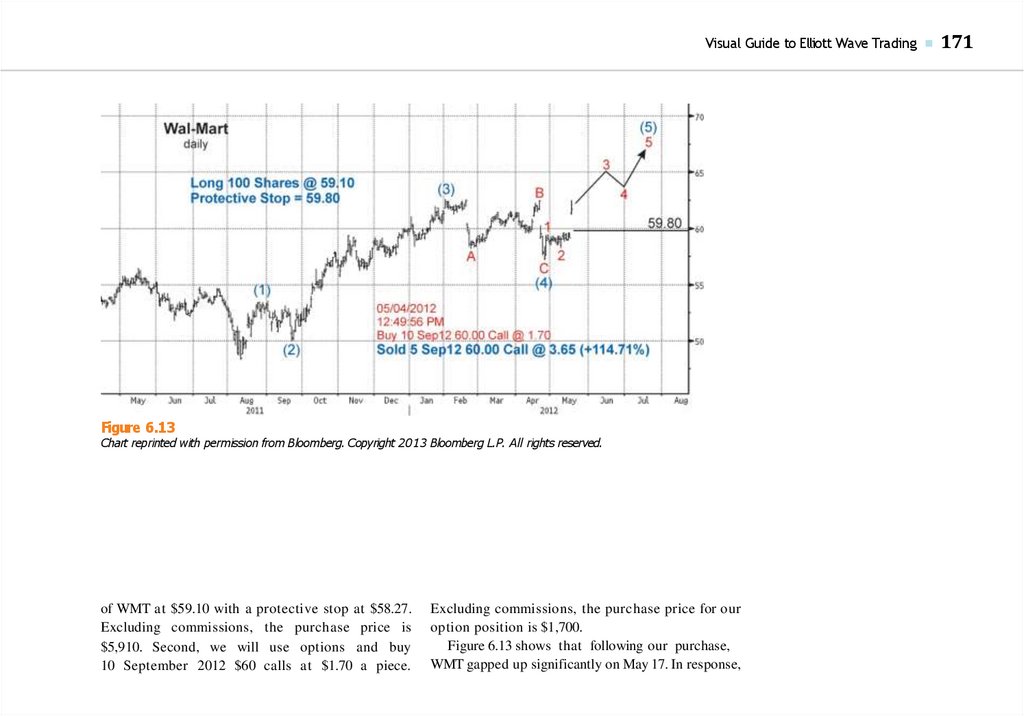
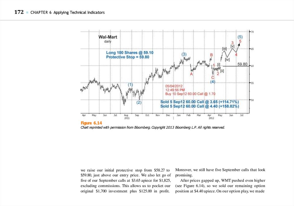

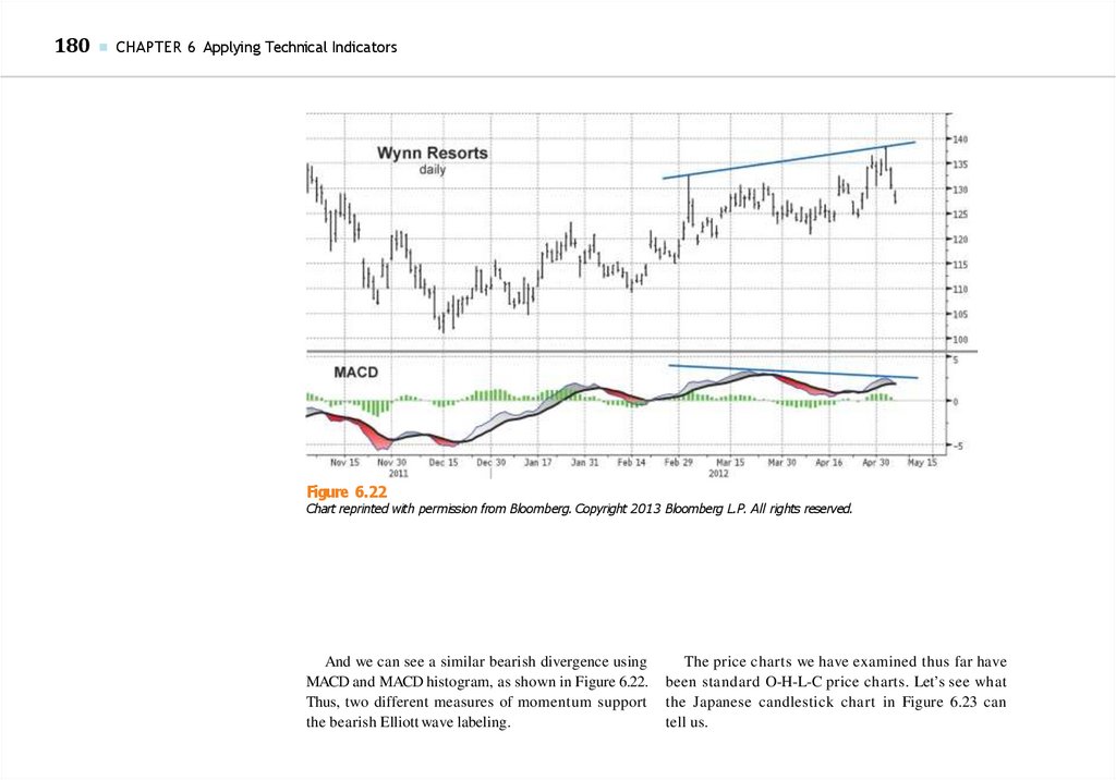
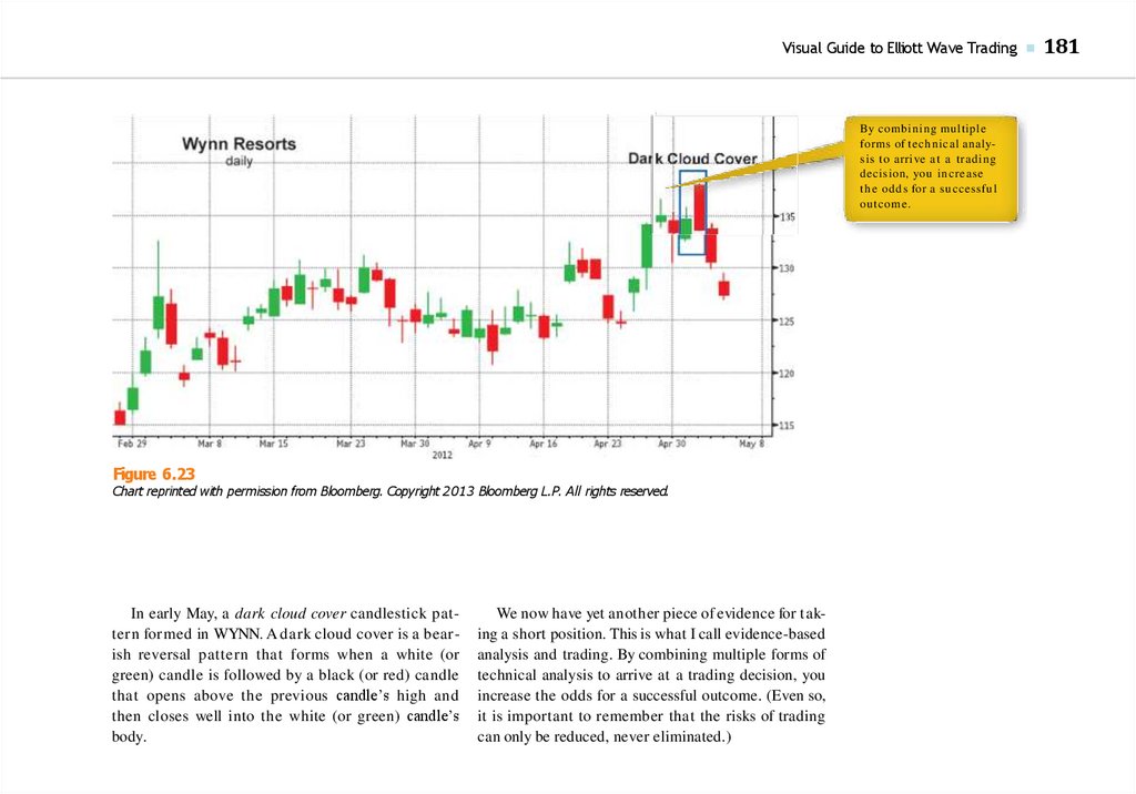


 Маркетинг
Похожие презентации:


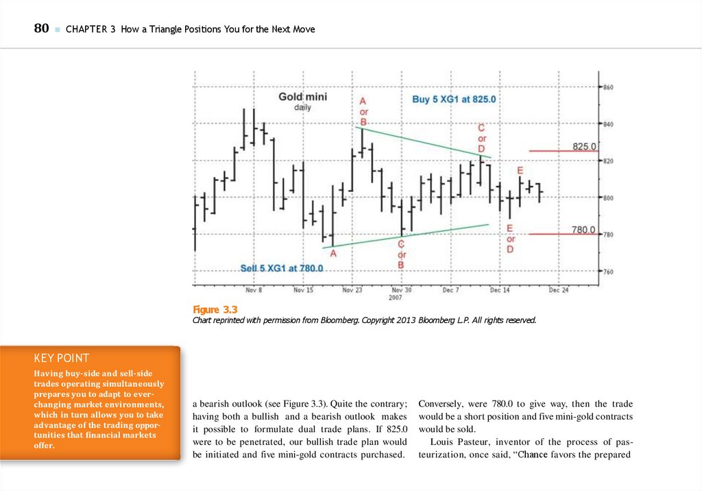
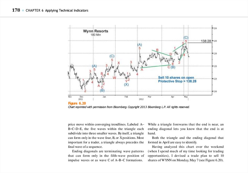
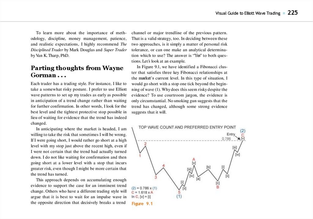
")


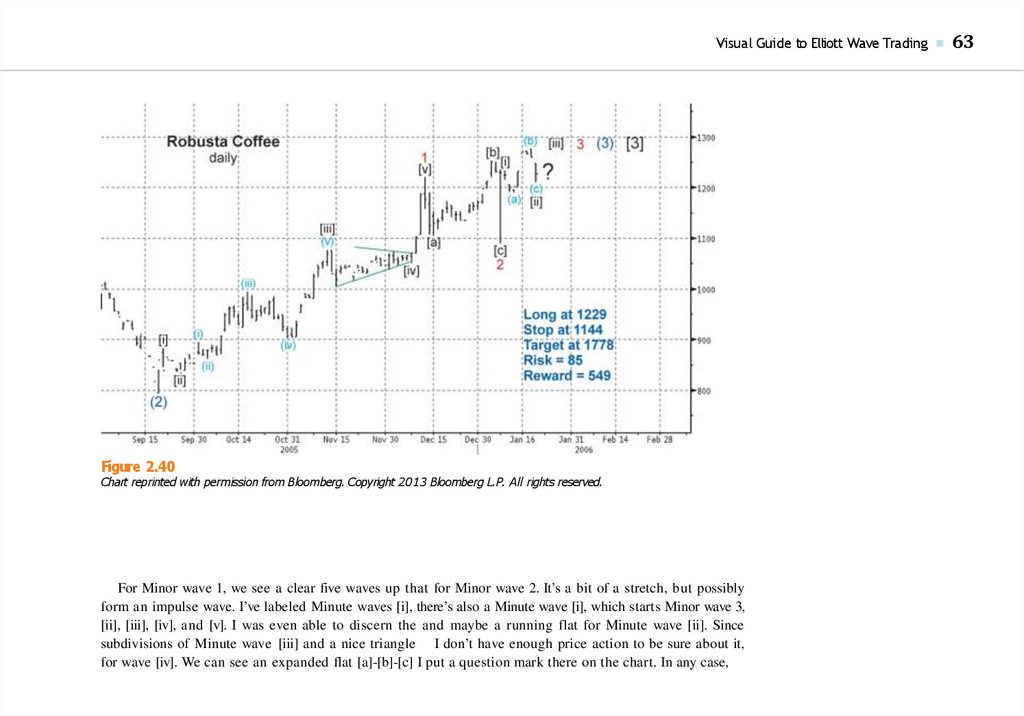
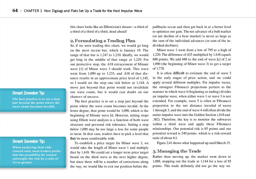
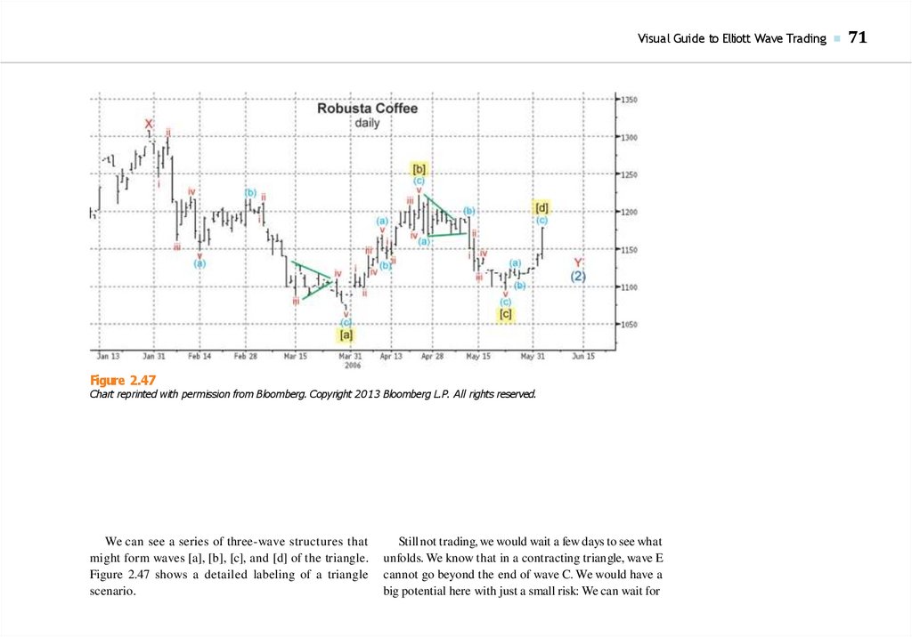
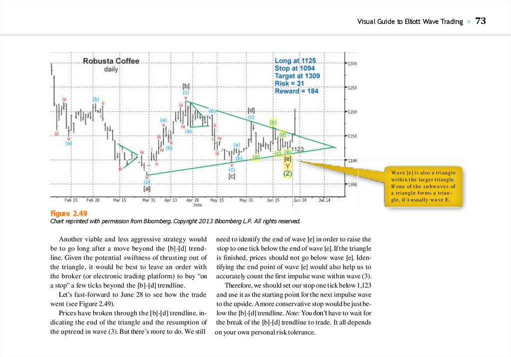
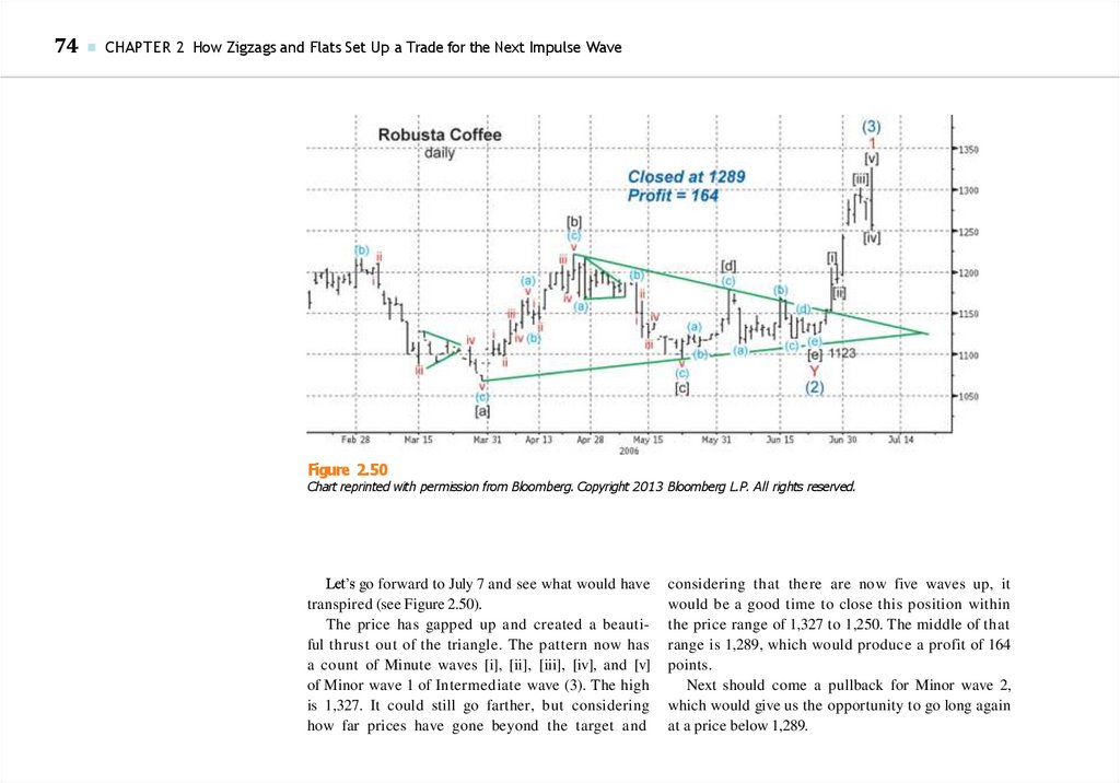
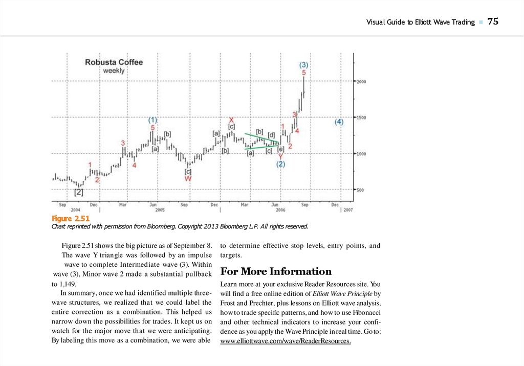
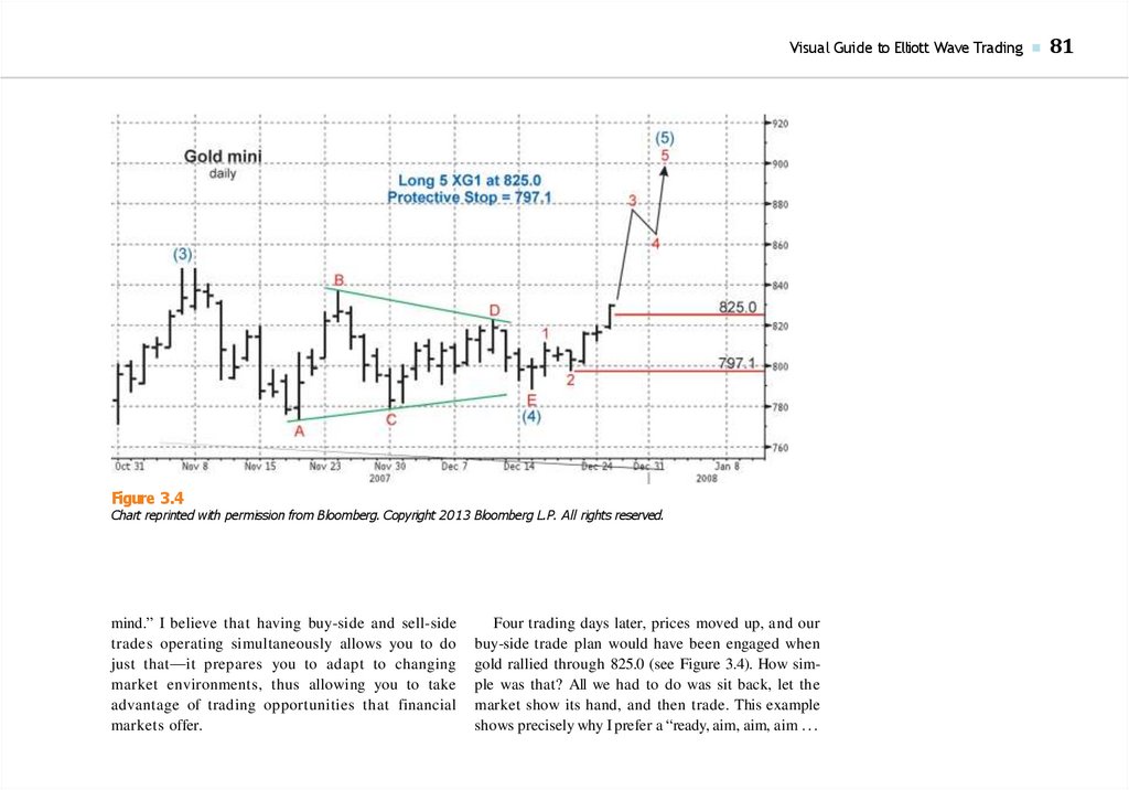
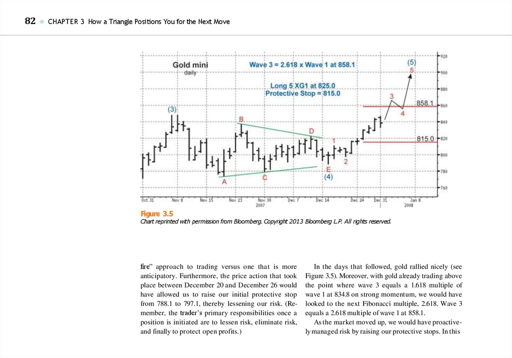
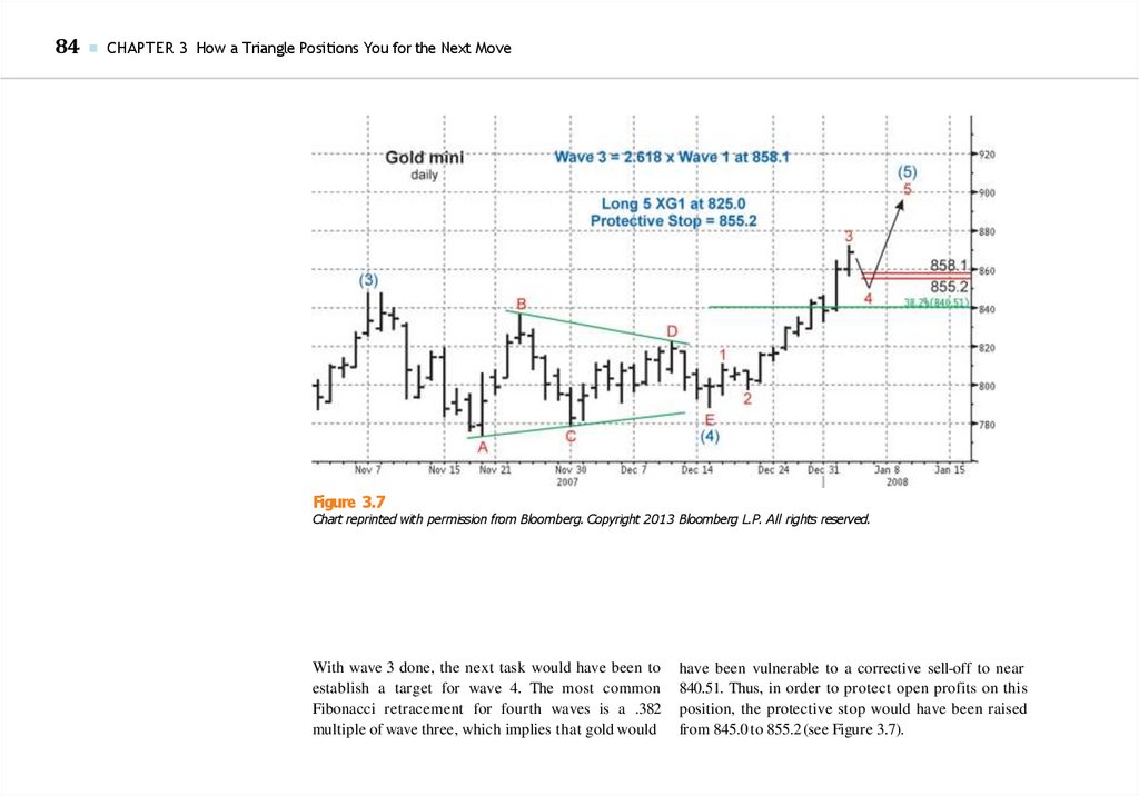
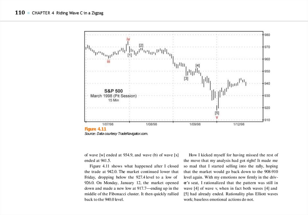
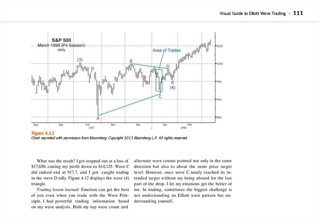
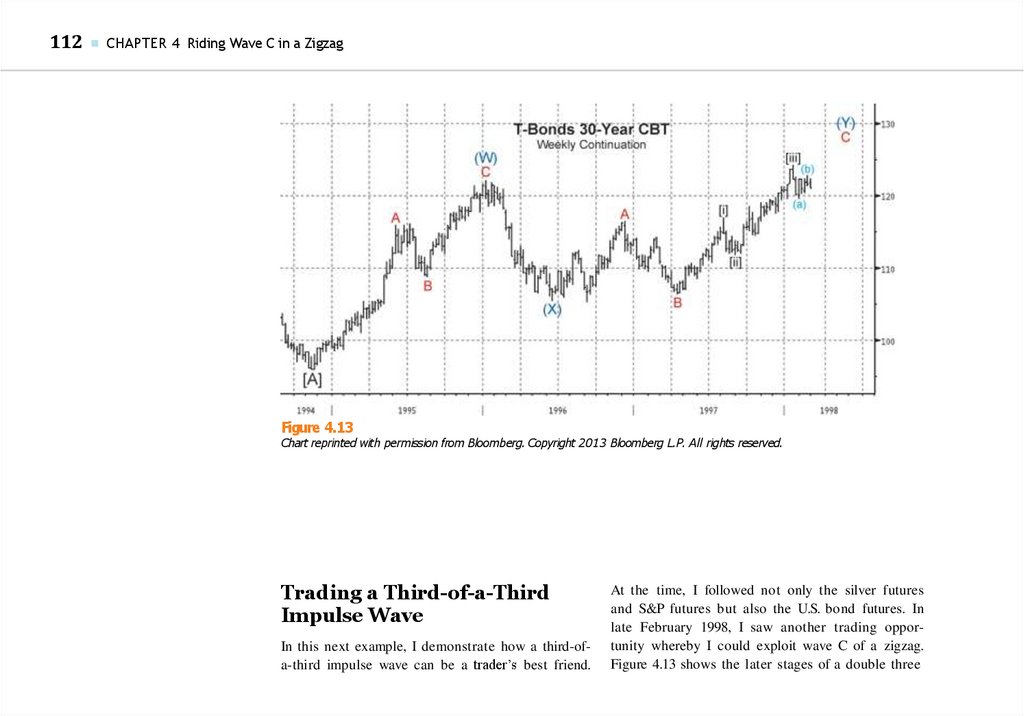
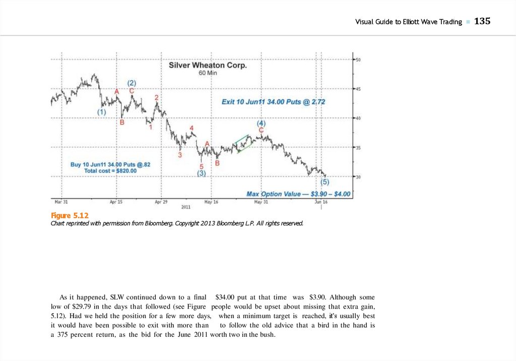
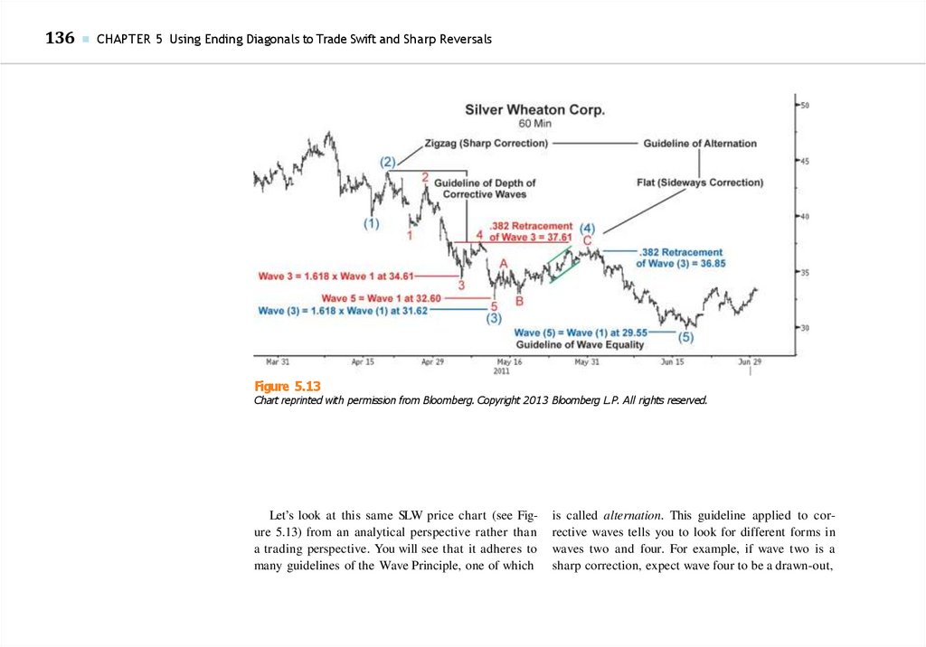
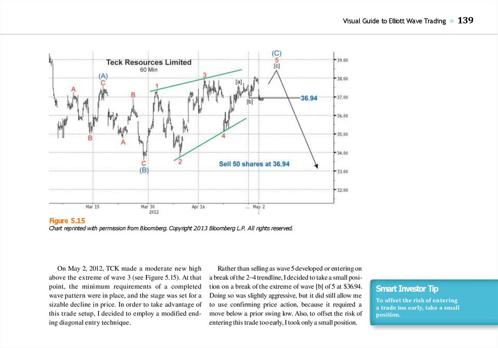
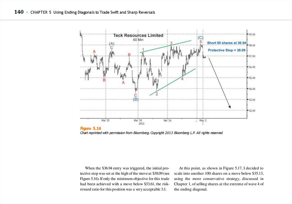
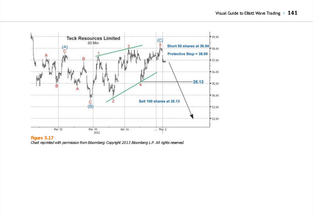
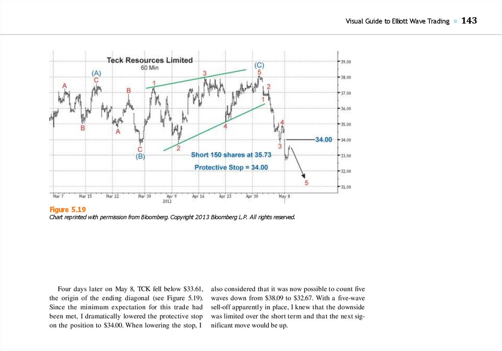
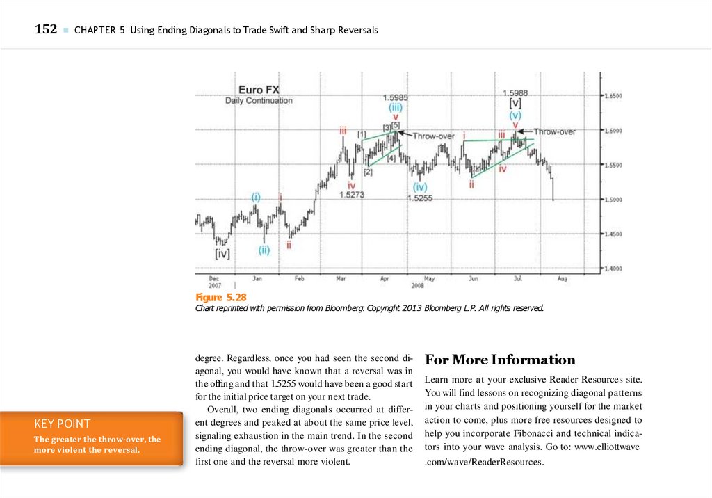
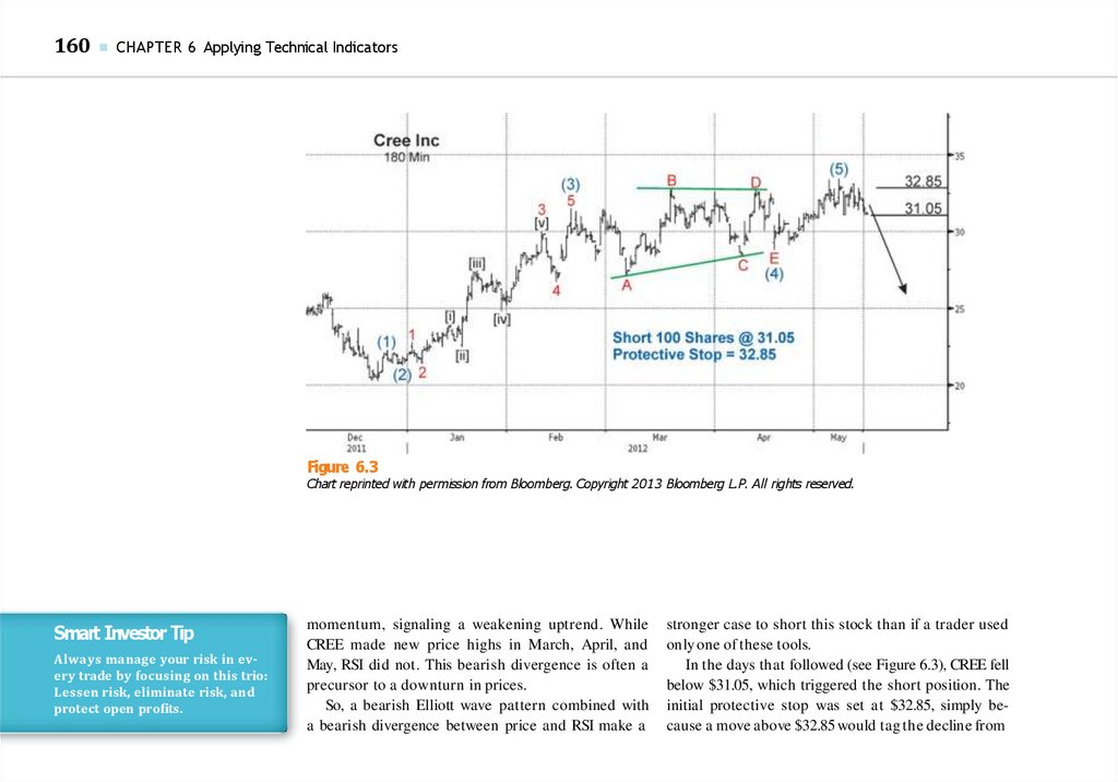
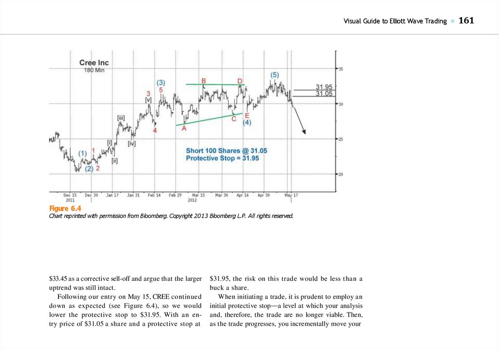
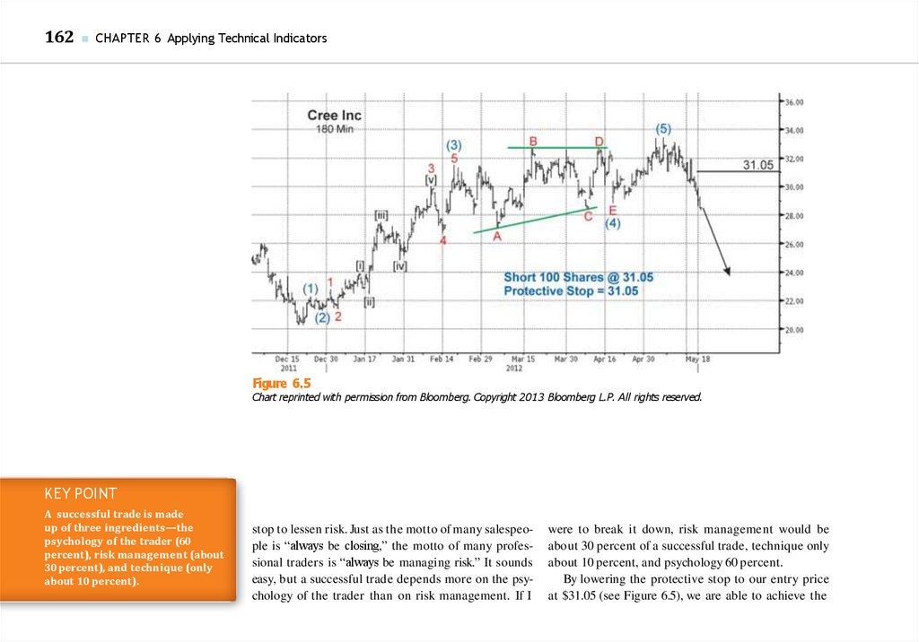
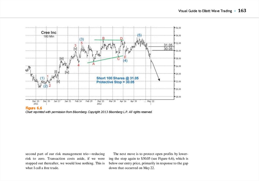
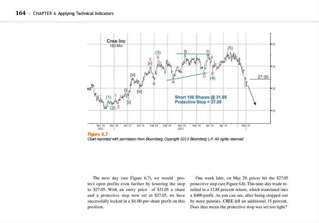
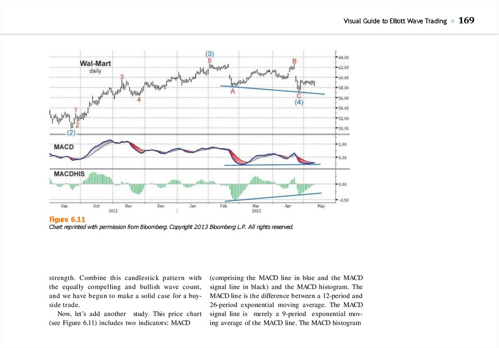
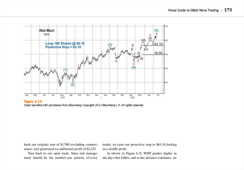
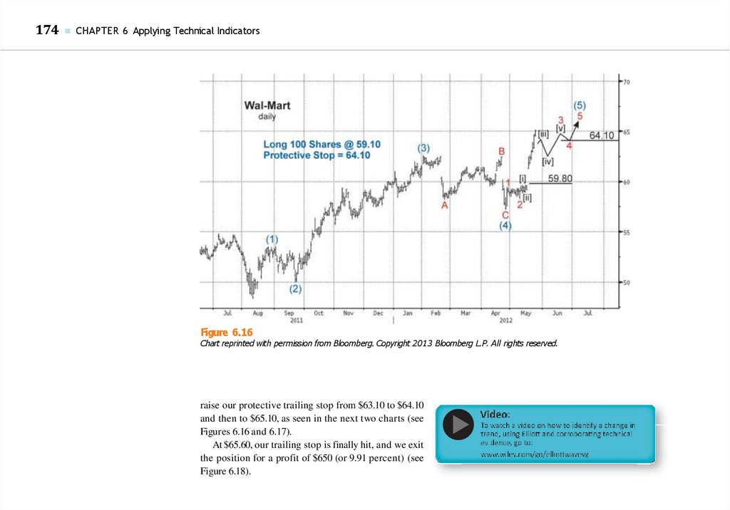
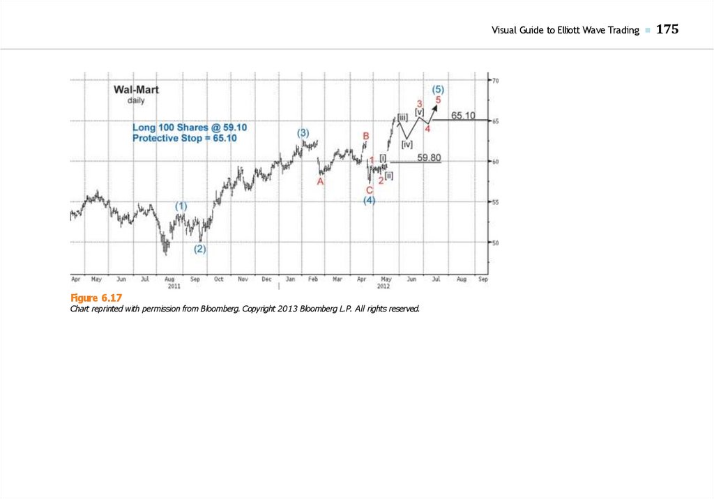
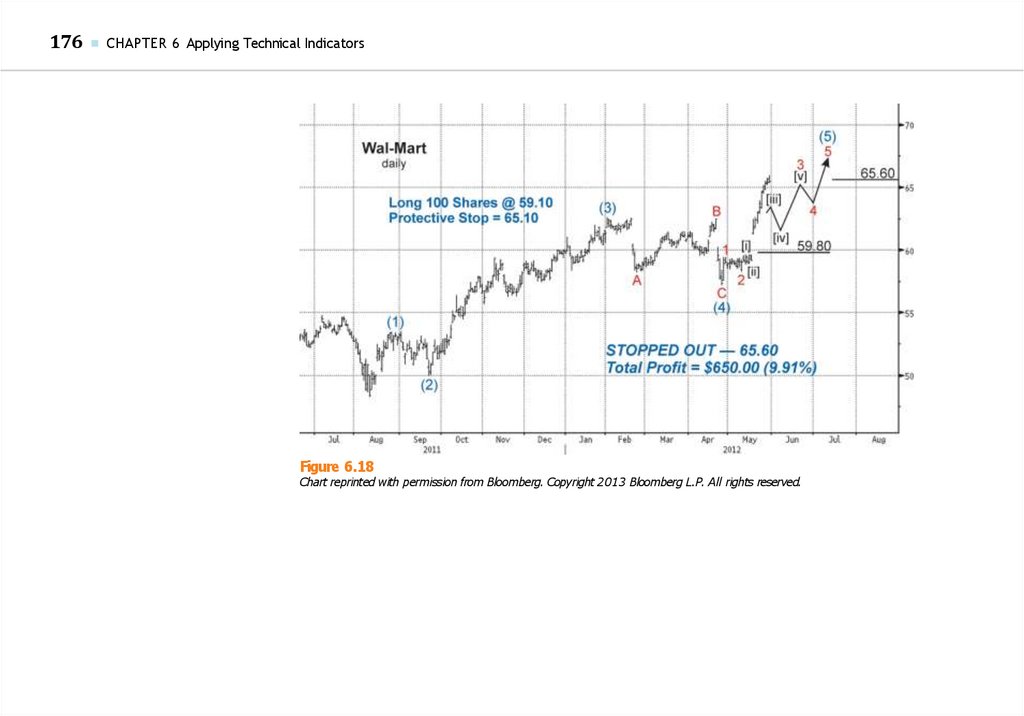
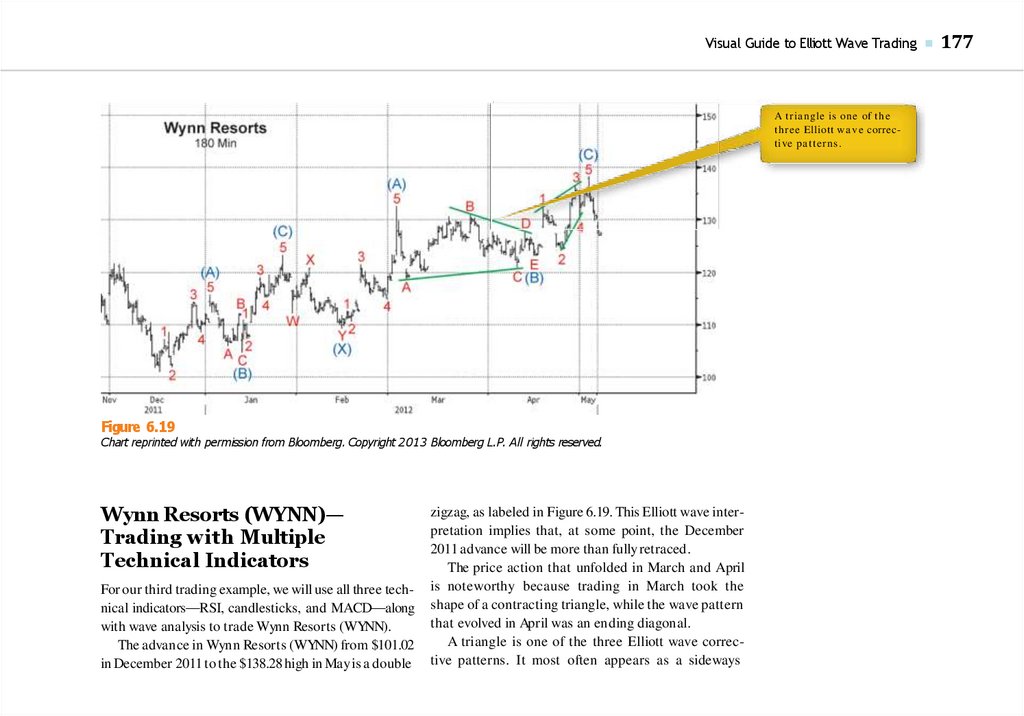
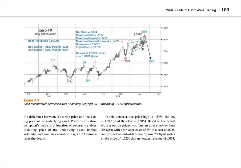
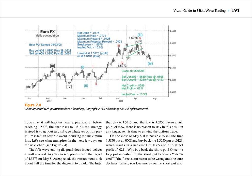
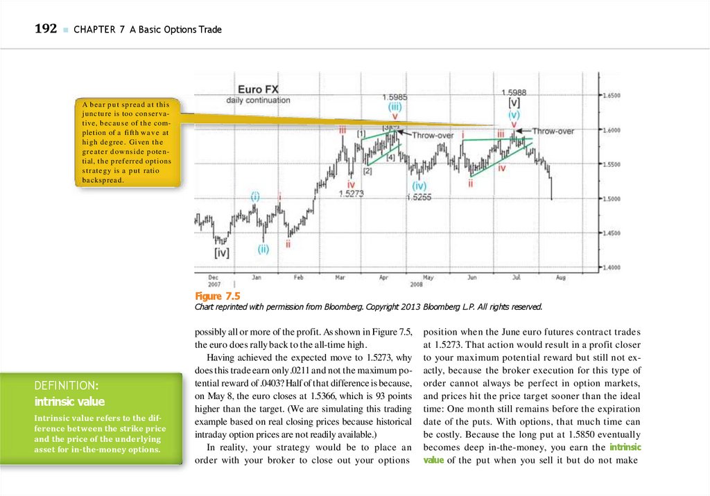
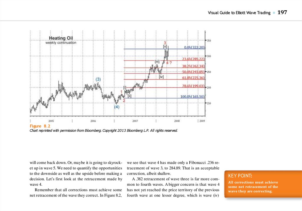
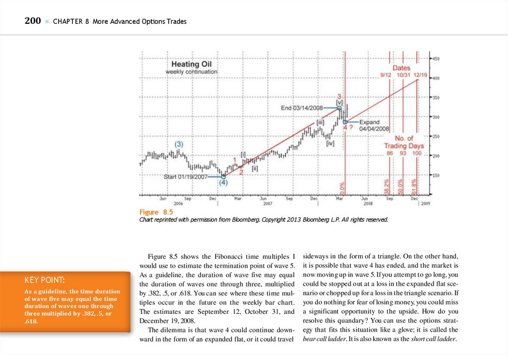
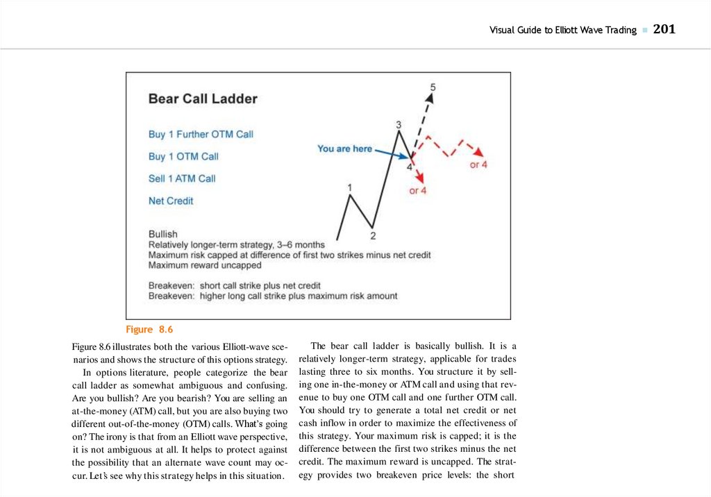
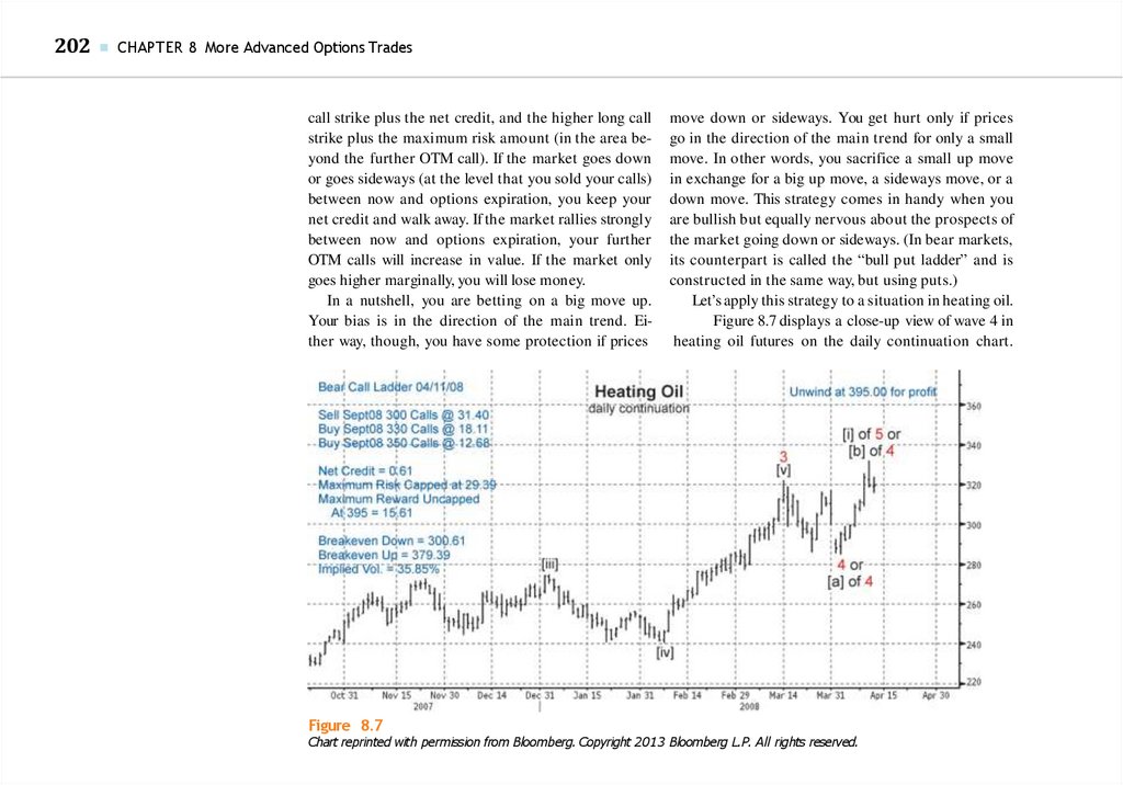
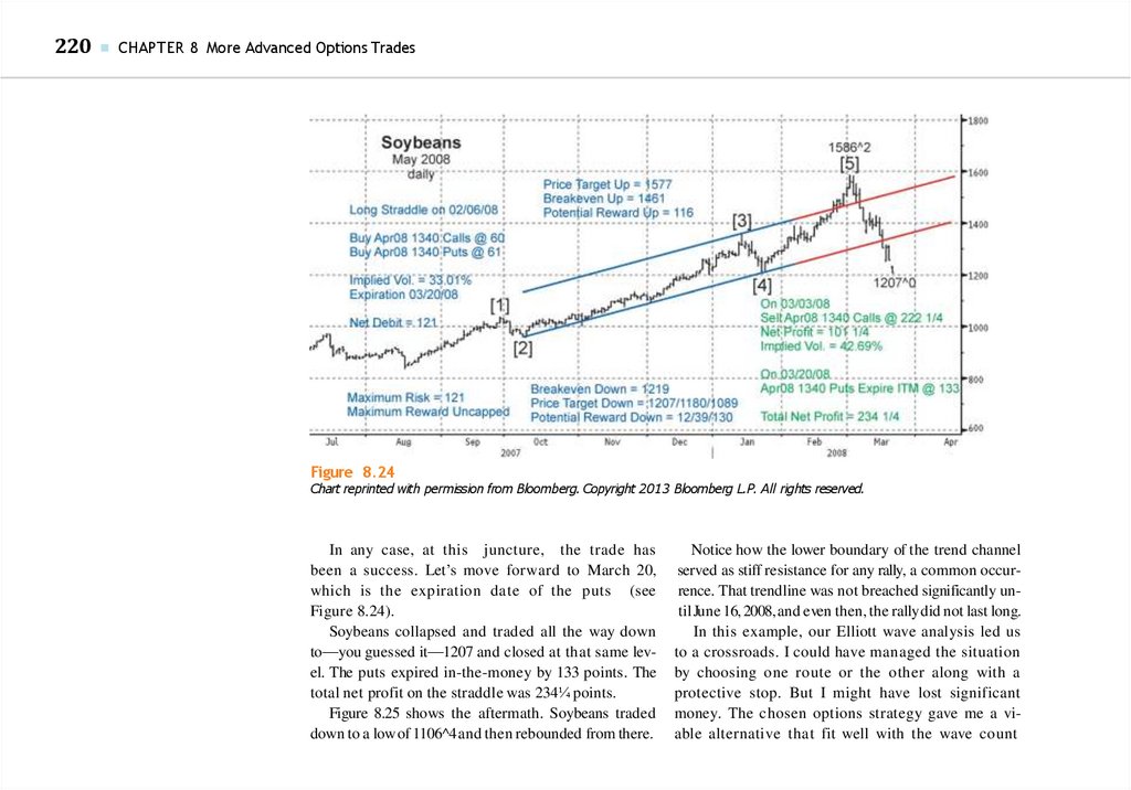
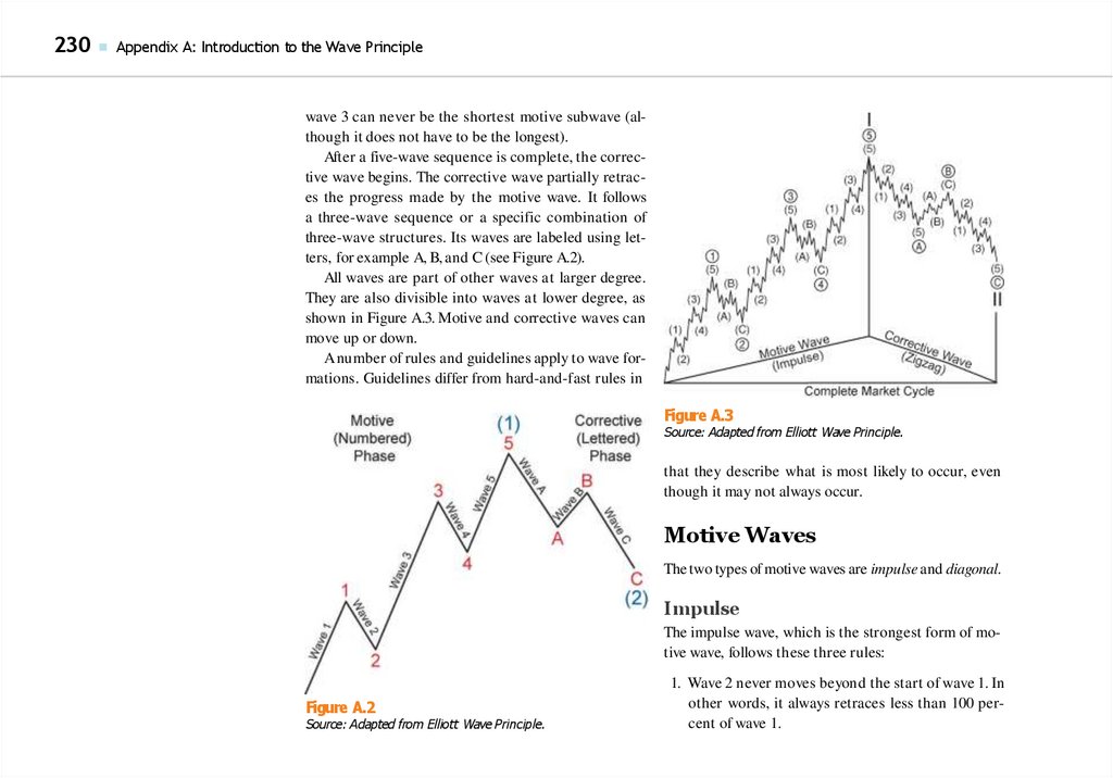
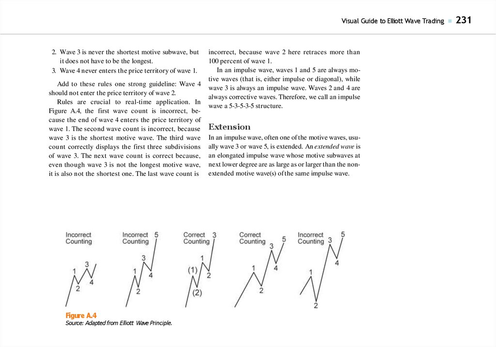
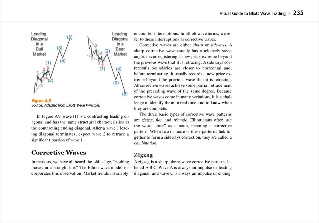
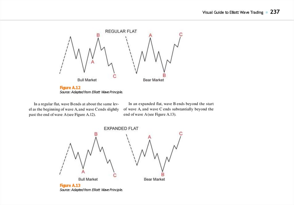
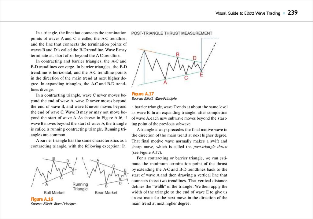
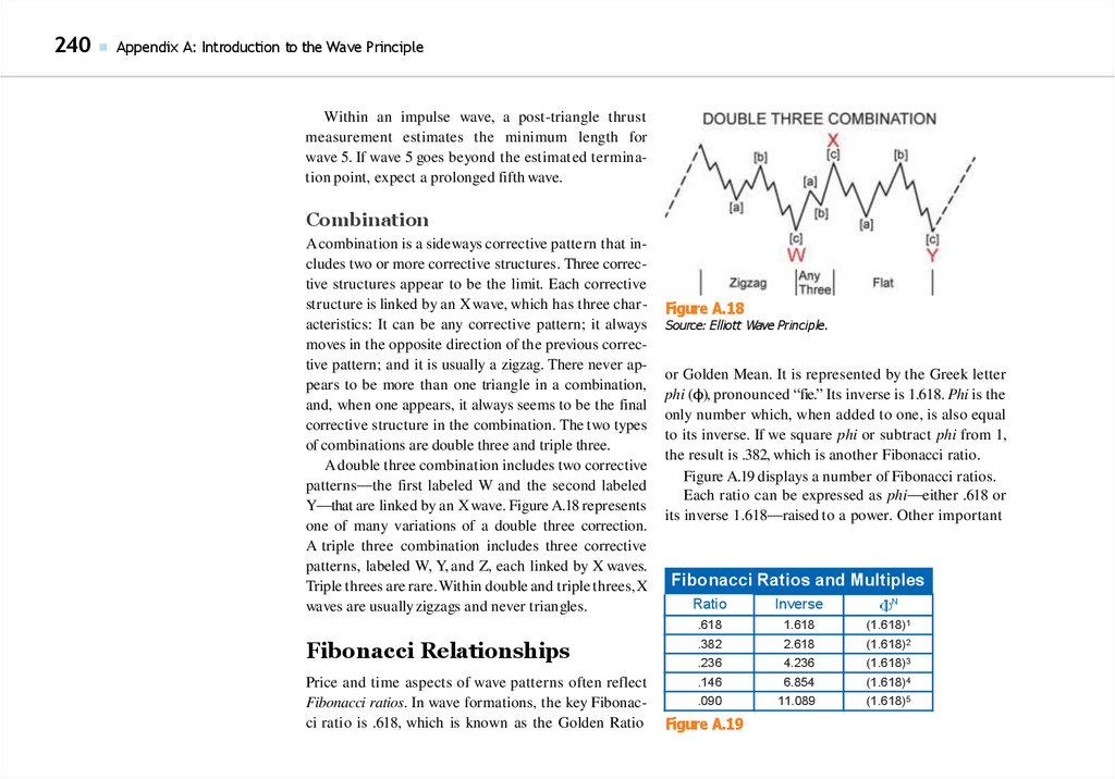
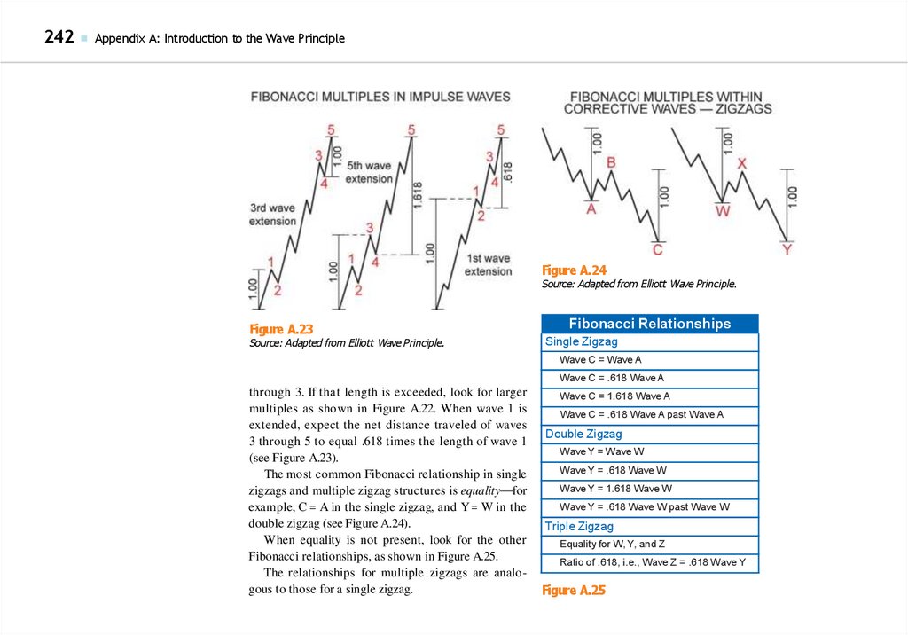
Visual Guide to Elliott Wave Trading
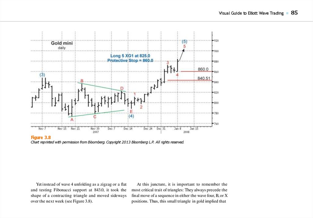
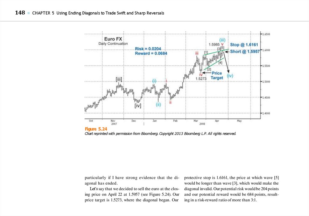
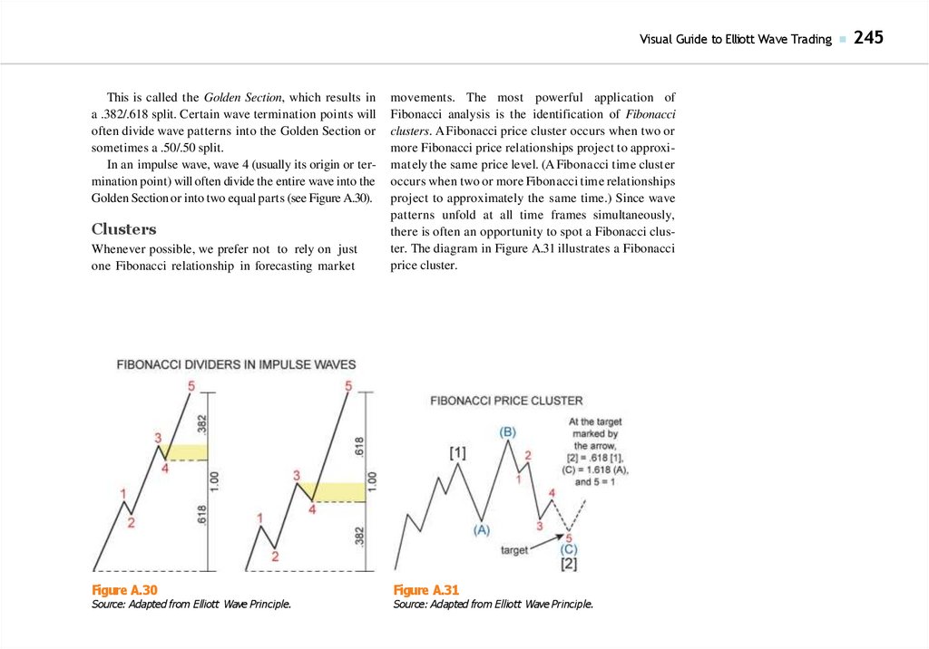
1.
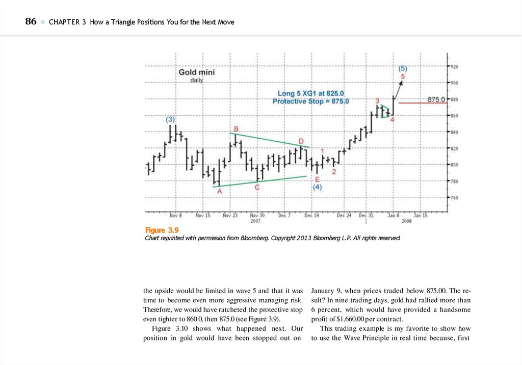
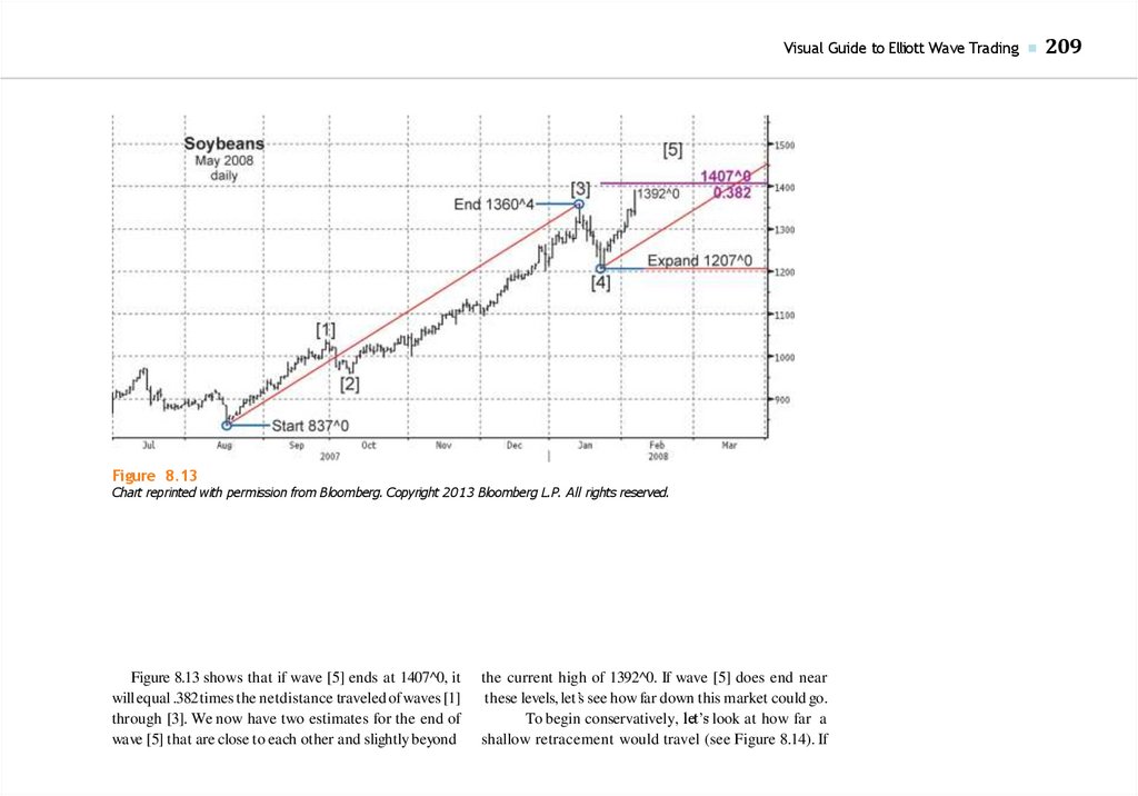
2.
3.
Visual Guide toElliott Wave Trading
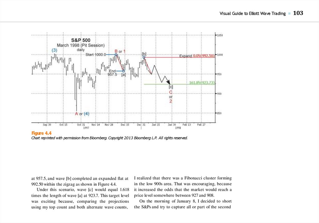
4.
Since 1996, Bloomberg Press has published books for finance professionals on investing, economics, and policyaffecting investors. Titles are written by leading practitioners and authorities, and have been translated into
more than 20 languages.
The Bloomberg Financial Series provides both core reference knowledge and actionable information for finance professionals. The books are written by experts familiar with the work flows, challenges, and demands of
investment professionals who trade the markets, manage money, and analyze investments in their capacity of
growing and protecting wealth, hedging risk, and generating revenue.
Books in the series include:
Visual Guide to Candlestick Charting by Michael Thomsett
Visual Guide to Municipal Bonds by Robert Doty
Visual Guide to Financial Markets by David Wilson
Visual Guide to Chart Patterns by Thomas N. Bulkowski
Visual Guide to ETFs by David Abner
Visual Guide to Options by Jared Levy
Visual Guide to Elliott Wave Trading by Wayne Gorman and Jeffrey Kennedy
For more information, please visit our Web site at www.wiley.com/go/bloombergpress.
5.
Visual Guide toElliott Wave Trading
Wayne Gorman
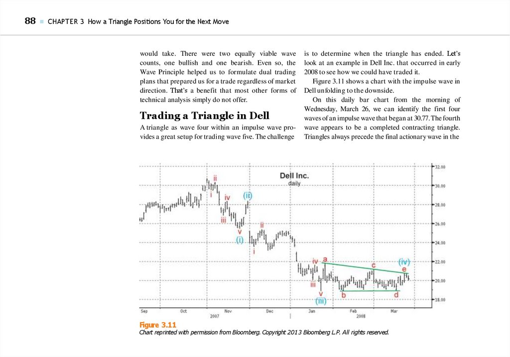
Jeffrey Kennedy
Foreword by Robert R. Prechter, Jr.
6.
Cover design: C. Wallace.Cover images: Waves by Peter Firus/iStockphoto, charts courtesy Wayne Gorman and Jeffrey Kennedy.
Copyright © 2013 by Elliott Wave International, Inc. All rights reserved.
Published by John Wiley & Sons, Inc., Hoboken, New Jersey.
Published simultaneously in Canada.
No part of this publication may be reproduced, stored in a retrieval system, or transmitted in any form or by any means,
electronic, mechanical, photocopying, recording, scanning, or otherwise, except as permitted under Section 107 or 108
of the 1976 United States Copyright Act, without either the prior written permission of the Publisher, or authorization
through payment of the appropriate per-copy fee to the Copyright Clearance Center, Inc., 222 Rosewood Drive, Danvers,
MA 01923, (978) 750-8400, fax (978) 646-8600, or on the Web at www.copyright.com. Requests to the Publisher for
permission should be addressed to the Permissions Department, John Wiley & Sons, Inc., 111 River Street, Hoboken, NJ
07030, (201) 748-6011, fax (201) 748-6008, or online at http://www.wiley.com/go/permissions.
Limit of Liability/Disclaimer of Warranty: While the publisher and authors have used their best efforts in preparing this
book, they make no representations or warranties with respect to the accuracy or completeness of the contents of this
book and specifically disclaim any implied warranties of merchantability or fitness for a particular purpose. No warranty
may be created or extended by sales representatives or written sales materials. The advice and strategies contained herein
may not be suitable for your situation. You should consult with a professional where appropriate. Neither the publisher
nor the authors shall be liable for any loss of profit or any other commercial damages, including but not limited to special,
incidental, consequential, or other damages.
For general information on our other products and services or for technical support, please contact our Customer Care
Department within the United States at (800) 762-2974, outside the United States at (317) 572-3993 or fax (317) 572-4002.
Wiley also publishes its books in a variety of electronic formats. Some content that appears in print may not be available
in electronic books. For more information about Wiley products, visit our web site at www.wiley.com.
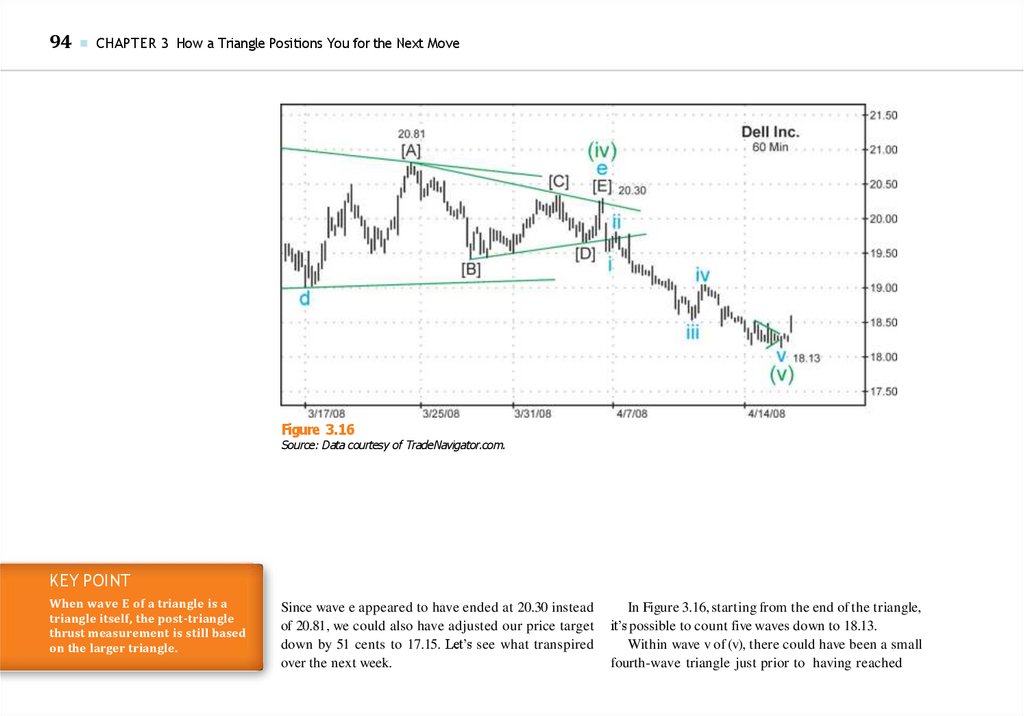
Library of Congress Cataloging-in-Publication Data:
Gorman, Wayne.
Visual guide to Elliott Wave trading / Wayne Gorman, Jeffrey Kennedy ; foreword by Robert R. Prechter, Jr.
pages cm.—(The Bloomberg financial series)
Includes index.
ISBN 978-1-118-44560-0 (paperback); ISBN 978-1-118-47953-7 (ebk);
ISBN 978-1-118-47950-6 (ebk); ISBN 978-1-118-47954-4 (ebk); ISBN 978-1-118-47951-3 (ebk);
ISBN 978-1-118-75405-4 (ebk); ISBN 978-1-118-75416-0 (ebk)
1. Speculation. 2. Stocks. 3. Elliott wave principle. I. Kennedy, Jeffrey (Business writer) II. Title.
HG6041.G593 2013
332.64’5—dc23
2013005664
Printed in the United States of America
10 9 8 7 6 5 4 3 2 1
7.
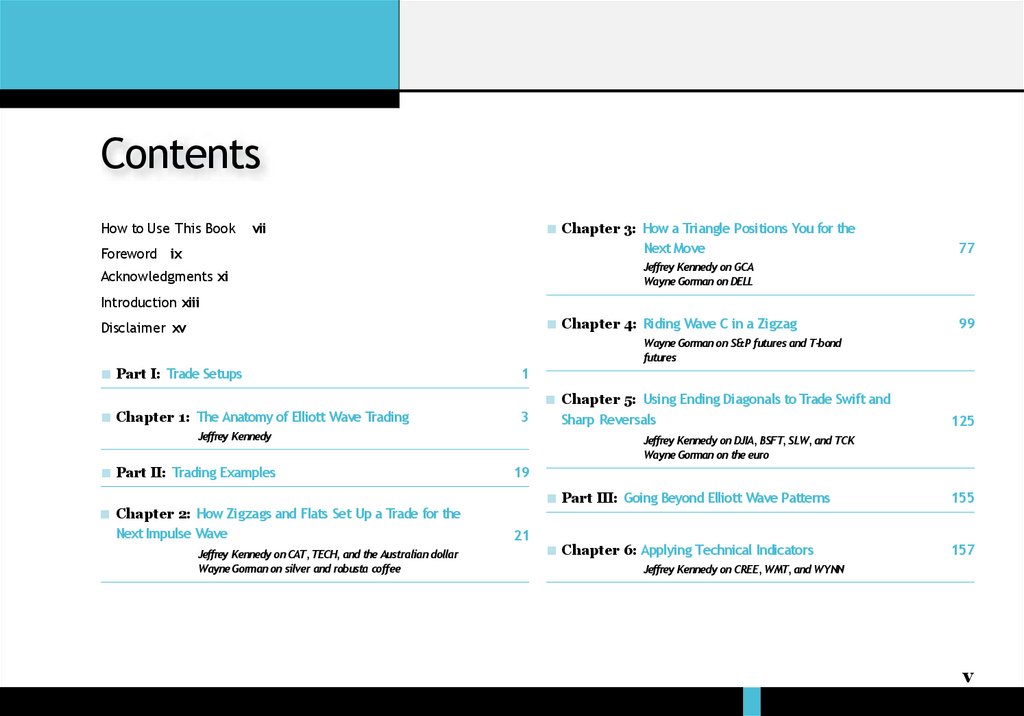
ContentsHow to Use This Book
■ Chapter 3: How a Triangle Positions You for the
Next Move
vii
Foreword ix
77
Jeffrey Kennedy on GCA
Wayne Gorman on DELL
Acknowledgments xi
Introduction xiii
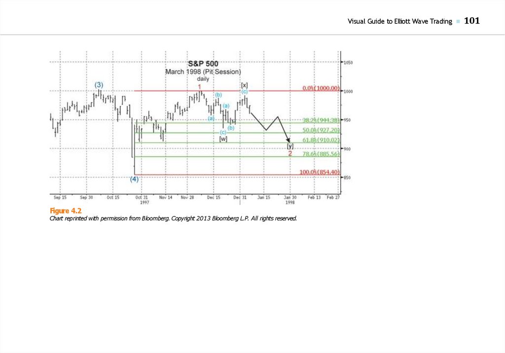
■ Chapter 4: Riding Wave C in a Zigzag
Disclaimer xv
Wayne Gorman on S&P futures and T-bond
futures
■ Part I: Trade Setups
1
■ Chapter 1: The Anatomy of Elliott Wave Trading
3
Jeffrey Kennedy
■ Part II: Trading Examples
■ Chapter 2: How Zigzags and Flats Set Up a Trade for the
Next Impulse Wave
Jeffrey Kennedy on CAT, TECH, and the Australian dollar
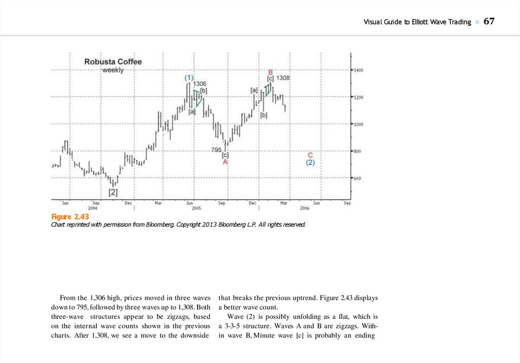
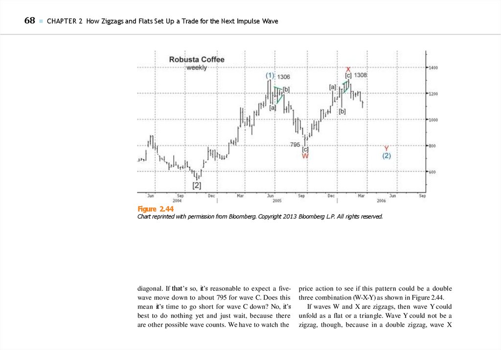
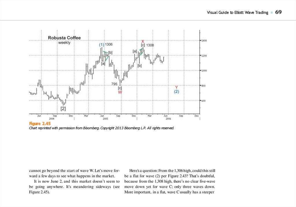
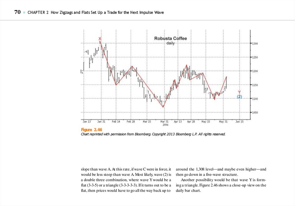
Wayne Gorman on silver and robusta coffee
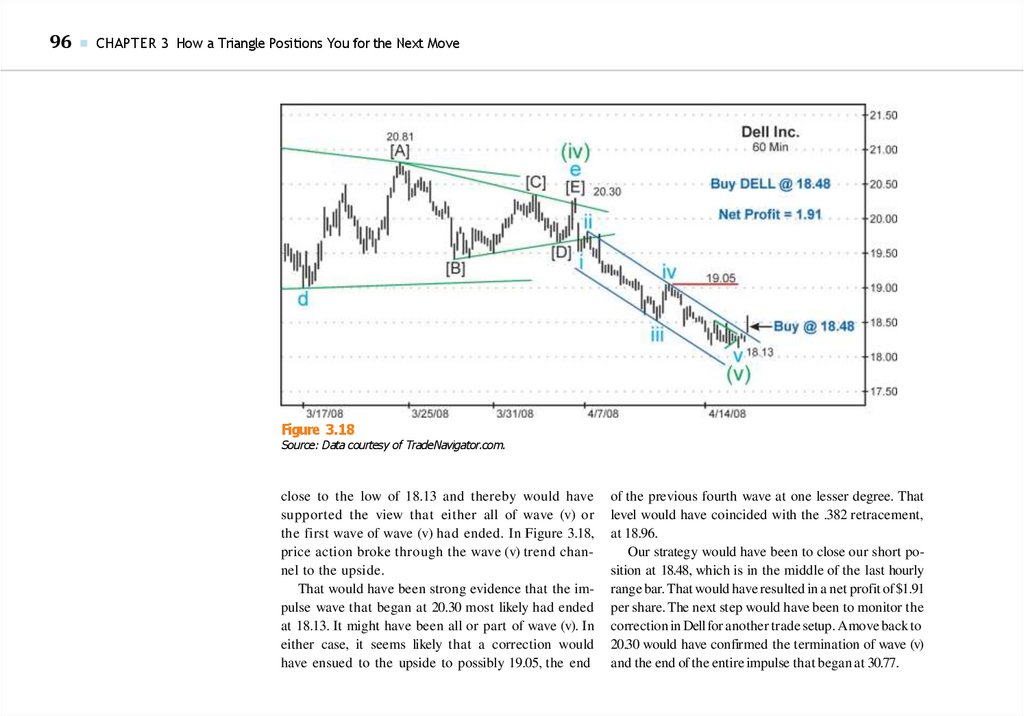
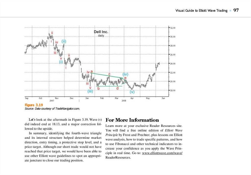
99
■ Chapter 5: Using Ending Diagonals to Trade Swift and
Sharp Reversals
125
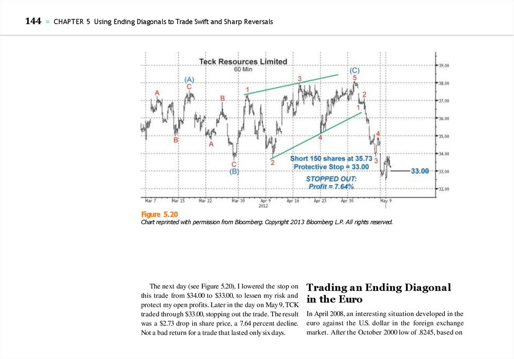
Jeffrey Kennedy on DJIA, BSFT, SLW, and TCK
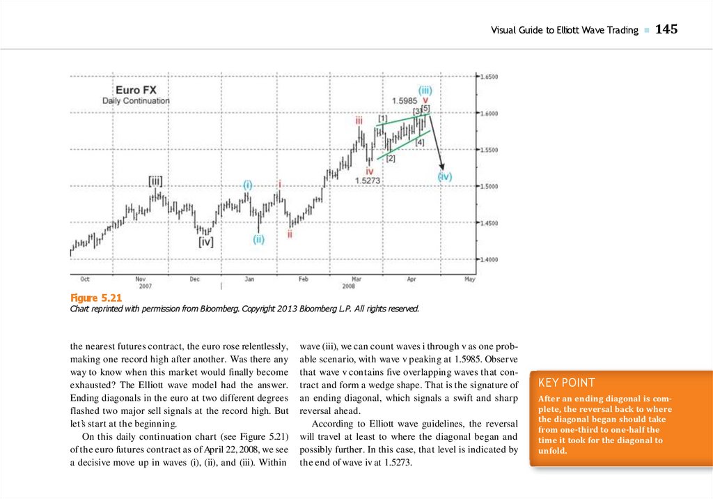
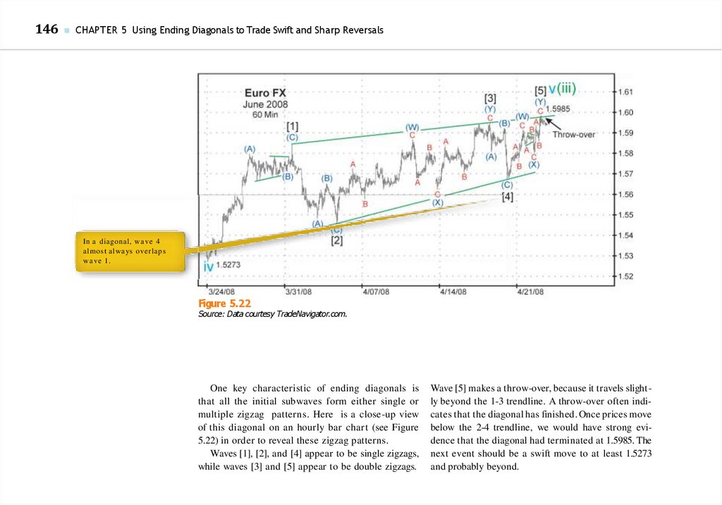
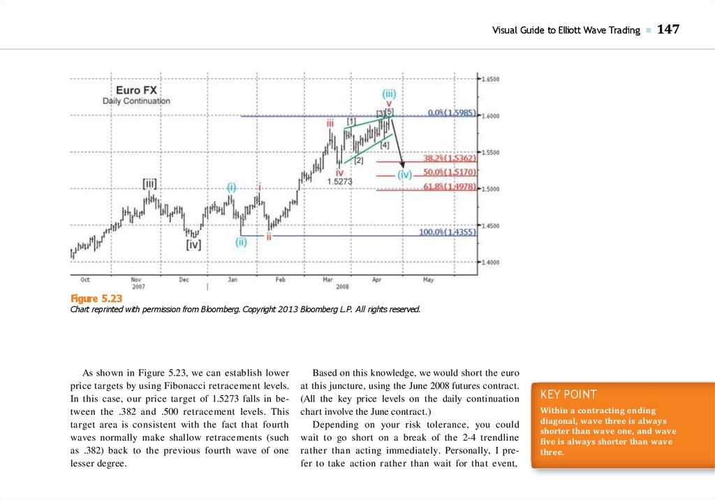
Wayne Gorman on the euro
19
21
■ Part III: Going Beyond Elliott Wave Patterns
155
■ Chapter 6: Applying Technical Indicators
157
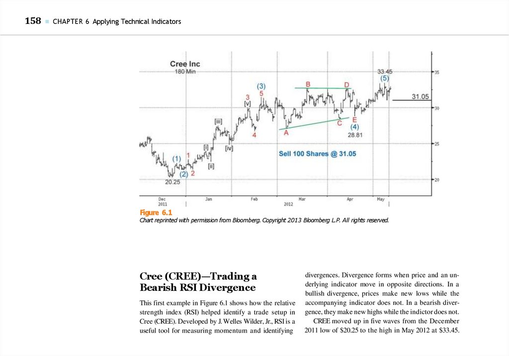
Jeffrey Kennedy on CREE, WMT, and WYNN
v
8.
vi■
Contents
■ Chapter 7: A Basic Options Trade
185
Wayne Gorman on the euro
■ Chapter 8: More Advanced Options
Trades
195
Wayne Gorman on heating oil and soybeans
■ Chapter 9: Parting Thoughts
223
Appendix A: Introduction to the Wave
Principle, by Wayne Gorman 229
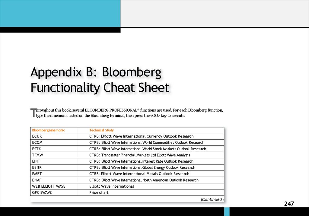
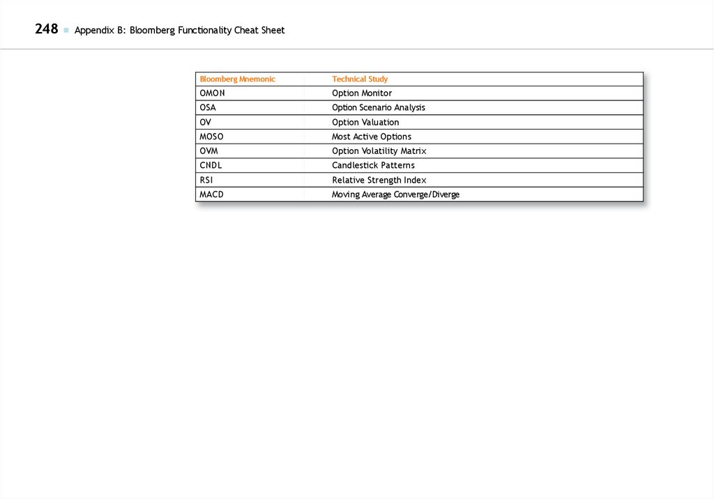
Appendix B: Bloomberg Functionality Cheat
Sheet 247
Glossary of Elliott Wave Terms 249
Educational Resources
About the Authors
Index 257
255
253
9.
How to Use This BookThe Visual Guide to . . . series is designed to be a comprehensive and easy-to-follow guide on today’s most
relevant finance and investing topics. All charts are
in full color and presented in a large format to make
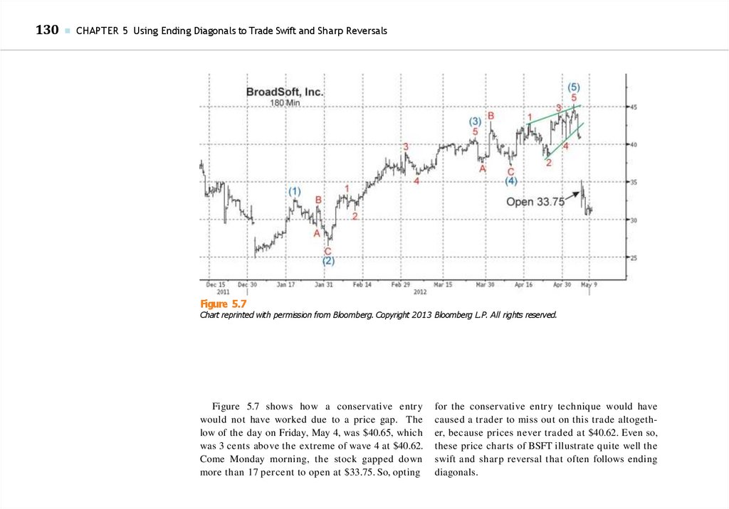
them easy to read and use. We’ve also included the
following elements to reinforce key information and
processes:
of relevant functions for the topics and tools
discussed
Go Beyond Print
■
Definitions: Terminology and technical concepts
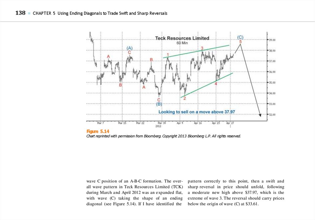
that arise in the discussion
■
Video Tutorials: To show concepts in action
■
■
Key Points: Critical ideas and takeaways from the
full text
Test Yourself: Multiple-choice or true/false quizzes
to reinforce your newfound knowledge and skills
■
Pop-Ups: Definitions for key terms
■
Bloomberg Functionality Cheat Sheet: For Bloomberg terminal users, a back-of-the-book summary
Every Visual Guide is also available as an e-book,
which includes the following features:
vii
10.
11.
ForewordFor many years, I have wanted to have my company produce a trading book based on the Elliott
wave model. As with markets, sometimes you have
to wait patiently for the time to be right. The time
is finally right, as two highly qualified Elliott-wave
traders have partnered to write a good book on
the subject.
Wayne Gorman, who ran a major trading desk at
Citibank and Westpac Banking Corporation, is head
of Educational Resources at Elliott Wave International
(EWI). Je rey Kennedy traded for a living and handles
Elliott Wave Junctures, EWI’s daily educational and
trade-identifying service. Both guys teach our trading
seminars. And they can write well, too.
This is not a book about how some market method
sets up perfect trades on paper. Wayne and Je walk
you step by step through their thinking process during a number of trades they took in real life. They also
present hypothetical setups that you might encounter
in your own market experience and show you how to
handle them. They aren’t easy layups but real conundrums that require thoughtful analysis and careful action. Unlike many experts, Wayne and Je aren’t shy
about relating some of their mistakes and what they
learned from them. When you read their discussions,
you will know they have walked the hard road of experience.
You will also realize how much work it takes to do
things right. Even if this book leads you to decide that
successful trading takes too much e ort, it will have
provided a service. Books that make trading look easy
actually cost you a lot of money in the end.
Frankly, most people are not cut out for trading.
No book can cure impulsiveness, timidity, laziness,
or a self-destructive personality. But this book does
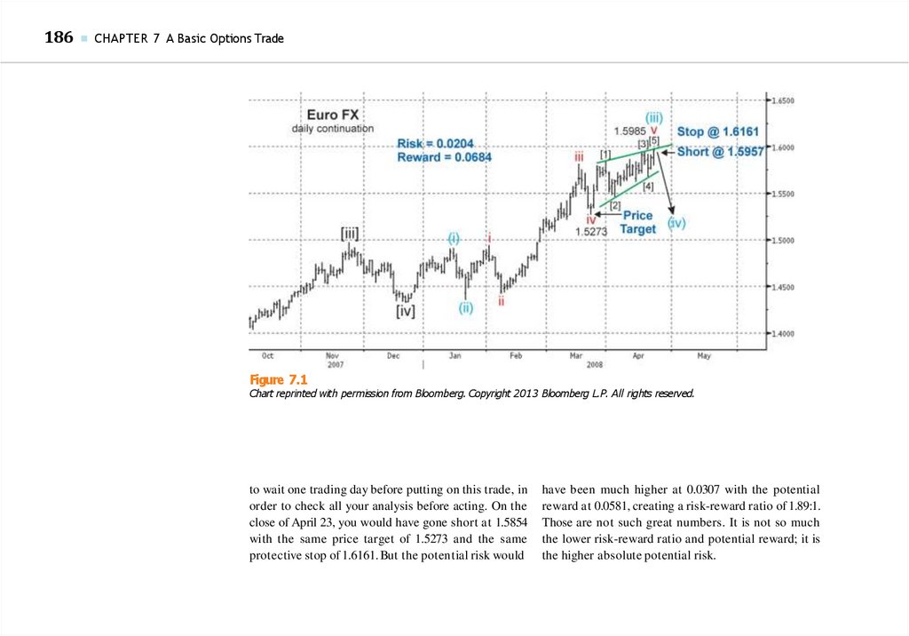
show you, very carefully, how two traders repeatedly
ix
12.
x■
Foreword
negotiate the minefield of the market and come out
alive and happy on the other side.
If you want to trade your own money for a living, if
you want to be employable as a trader, if you just want
to trade the occasional ideal setup, or even if your goal
is simply to stop losing money in the markets, you are
in the right place.
Successful trading takes work, discipline, and
smarts. With those three things, you’re mostly there.
The final thing you need is knowledge—that’s what
this book provides.
Robert R. Prechter, Jr.
Elliott Wave International
13.
AcknowledgmentsWe want to thank our colleagues for their valuable assistance in producing this volume: Sally Webb, Paula
Roberson, Susan Walker, Cari Dobbins, Dave Allman, Debbie Hodgkins, Bob Prechter, Will Rettiger, Michael
McNeilly, and Pam Greenwood.
xi
14.
15.
IntroductionWelcome! Visual Guide to Elliott Wave Trading is a
must-have book on how to use the Elliott Wave Principle—how to use it to find trades, assess trades, enter
trades, manage trades throughout by raising or lowering protective stops, and exit trades.
Visual Guide to Elliott Wave Trading assumes a basic
familiarity with the Wave Principle and its application.
Much like a strategy book for chess assumes a basic
knowledge of how the pieces move around the board,
this book assumes a basic knowledge of the various patterns of the Wave Principle and how they fit together.
If you are already an experienced Elliott wave practitioner and simply need a refresher, the Appendix reviews these basic building blocks and their structures.
If you are a complete newcomer or you want a
more in-depth review, we suggest you consult the
free resources and access your free copy of the Wall
Street classic Elliott Wave Principle by Frost and
Prechter at your exclusive Reader Resources site:
www.elliottwave.com/wave/ReaderResources.
Both of us have traded for a living at one time or
another. Each of us during those times used the Elliott
Wave Principle as our primary discipline. Visual Guide
to Elliott Wave Trading walks you through a highly personal journey of our thought processes throughout
each trade: what we looked at, what we ignored, what
we did right, and what we did wrong.
We do not present perfect-world examples that will
leave you convinced that you can trade your way to
wealth in 30 minutes while golfing the rest of the day.
Rather, we have tried to produce a realistic trading
book, warts and all, recognizing that while there may
be no one perfect way to trade, there are various ways
to trade successfully using the Wave Principle as your
primary discipline.
We hope you enjoy Visual Guide to Elliott Wave
Trading. Let’s get started.
Wayne Gorman and Je rey Kennedy
xiii
16.
17.
DisclaimerThe trading examples throughout this book are solely for the purpose of demonstrating the mechanics of
applying the Wave Principle. The profit or loss outcomes are not meant in any way to represent or imply a
particular rate of success or return on capital.
xv
18.
19.
Visual Guide toElliott Wave Trading
20.
21.
PAR TTrade Setups
22.
23.
CH AP TE RThe Anatomy of
Elliott Wave Trading
W
hen teaching the Wave Principle, I begin each
class by stating that analysis and trading represent two different skill sets. Although you may be a
talented analyst, that does not mean you will be a successful trader and vice versa. I learned the hard way
over many years that skilled analysis is a mastery of observation, while successful trading is a mastery of self.
When it comes to trading, there is no right way or
wrong way—only your way. One trader’s tolerance
for risk will be starkly different from another’s, just
as time frame, portfolio size, and markets traded will
also be different. Thus, the guidelines offered within
this chapter on how to trade specific Elliott wave patterns are just that—guidelines, but ones that have
served me well for many years.
My best advice to you as you look for a trading
opportunity is to start your search by asking the
question, “Do I see a wave pattern I recognize?” You
should look for one of the five core Elliott wave patterns: impulse wave, ending diagonal, zigzag, flat, or
triangle. These forms will become the basis of all your
trade setups once you learn to identify them quickly
and with confidence.
An even simpler question to ask is, “Do I see either
a motive wave or a corrective wave?” Motive waves
define the direction of the trend. There are two kinds
of motive waves: impulse waves and ending diagonals.
Corrective waves travel against the larger trend. The
three kinds of corrective waves are zigzags, flats, and
triangles. If all you do is identify a motive wave versus
a corrective wave correctly, you can still identify some
useful trade setups.
In this chapter, we will examine how to use key
components of analysis and trading to help you
KEY POINT
Analysis is a mastery of observation, while successful trading is a
mastery of self.
3
24.
4■
CHAPTER 1 The Anatomy of Elliott Wave Trading
become a better Elliottician and a consistently successful trader. Specifically, we will examine how the
Wave Principle improves trading, which waves are
the best to trade, which guidelines to use for trading
specific Elliott wave patterns, and why the psychology
of trading and risk management—what I call the
neglected essentials—are important.
How the Wave Principle
Improves Trading
Every trader, every analyst, and every technician has
favorite techniques to use when trading. Let’s go over
why the Wave Principle is mine.
How the Wave Principle Improves
Upon Traditional Technical Studies
There are three categories of technical studies: trendfollowing indicators, oscillators, and sentiment indicators. Trend-following indicators include moving
averages, Moving Average Convergence-Divergence
(MACD), and Directional Movement Index (ADX). A
few of the more popular oscillators many traders use
today are stochastics, rate-of-change, and the Commodity Channel Index (CCI). Sentiment indicators
include put-call ratios and Commitment of Traders
report data.
Technical studies like these do a good job of illuminating the way for traders, yet they each fall short
for one major reason: They limit the scope of a trader’s
understanding of current price action and how it relates to the overall picture of a market. For example,
let’s say the MACD reading in XYZ stock is positive,
indicating the trend is up. That’s useful information,
but wouldn’t it be more useful if it could also help to
answer these questions: Is this a new trend or an old
trend? If the trend is up, how far will it go?
Most technical studies simply don’t reveal pertinent information such as the maturity of a trend and
a definable price target—but the Wave Principle does.
Five Ways the Wave Principle
Improves Trading
Here are five ways the Wave Principle can benefit you
and improve your trading:
1. The Wave Principle identifies the trend.
2. It identifies countertrend price moves within the
larger trend.
3. It determines the maturity of the trend.
4. It provides high-confidence price targets.
5. It provides specific points of invalidation.
1. Identifying the Trend
“. . . action in the same direction as the one larger
trend develops in five waves. . . .”
—Elliott Wave Principle by Frost and Prechter
The Wave Principle identifies the direction of the
dominant trend. A five-wave advance identifies the
25.
Visual Guide to Elliott Wave Tradingoverall trend as up. Conversely, a five-wave decline determines that the larger trend is down. Why is this information important? Because it is easier to trade in
the direction of the dominant trend, since it is the path
of least resistance and undoubtedly explains the saying,
“The trend is your friend.” I find trading in the direction of
the trend much easier than attempting to pick tops and
bottoms within a trend, which is a difficult endeavor and
one that is virtually impossible to do consistently.
2. Identifying the Countertrend
“.. . reaction against the one larger trend develops in
three waves. . . .”
—Elliott Wave Principle by Frost and Prechter
The Wave Principle also identifies countertrend
moves. The three-wave pattern is a corrective response to the preceding impulse wave. Knowing that
a recent move in price is merely a correction within
a larger trending market is especially important for
traders because corrections give traders opportunities to position themselves in the direction of the larger trend of a market.
Being aware of the three basic Elliott wave corrective patterns—zigzags, flats, and triangles—enables
you to buy pullbacks in an uptrend and to sell bounces in a downtrend, which is a proven and consistently
successful trading strategy. Know what countertrend
price moves look like, and you can find opportunities
to rejoin the trend.
3. Determining the Maturity of a Trend
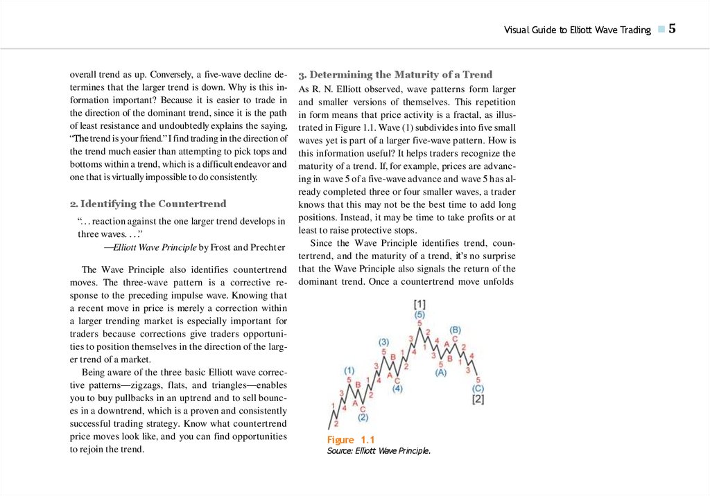
As R. N. Elliott observed, wave patterns form larger
and smaller versions of themselves. This repetition
in form means that price activity is a fractal, as illustrated in Figure 1.1. Wave (1) subdivides into five small
waves yet is part of a larger five-wave pattern. How is
this information useful? It helps traders recognize the
maturity of a trend. If, for example, prices are advancing in wave 5 of a five-wave advance and wave 5 has already completed three or four smaller waves, a trader
knows that this may not be the best time to add long
positions. Instead, it may be time to take profits or at
least to raise protective stops.
Since the Wave Principle identifies trend, countertrend, and the maturity of a trend, it’s no surprise
that the Wave Principle also signals the return of the
dominant trend. Once a countertrend move unfolds
Figure 1.1
Source: Elliott Wave Principle.
■5
26.
6■
CHAPTER 1 The Anatomy of Elliott Wave Trading
in three waves (A-B-C), this structure can signal the
point where the dominant trend has resumed, namely, once price action exceeds the extreme of wave B.
Knowing precisely when a trend has resumed brings
an added benefit: It increases the likelihood of a successful trade, which is further enhanced when accompanied by traditional technical studies.
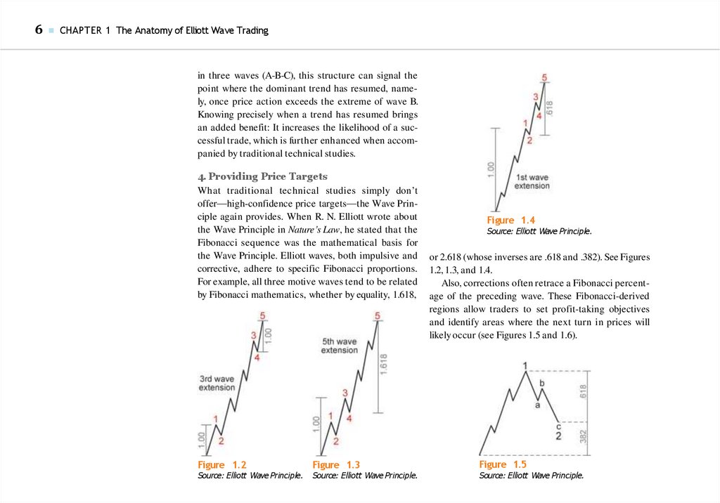
4. Providing Price Targets
What traditional technical studies simply don’t
offer—high-confidence price targets—the Wave Principle again provides. When R. N. Elliott wrote about
the Wave Principle in Nature’s Law, he stated that the
Fibonacci sequence was the mathematical basis for
the Wave Principle. Elliott waves, both impulsive and
corrective, adhere to specific Fibonacci proportions.
For example, all three motive waves tend to be related
by Fibonacci mathematics, whether by equality, 1.618,
Figure 1.2
Figure 1.3
Source: Elliott Wave Principle.
Source: Elliott Wave Principle.
Figure 1.4
Source: Elliott Wave Principle.
or 2.618 (whose inverses are .618 and .382). See Figures
1.2, 1.3, and 1.4.
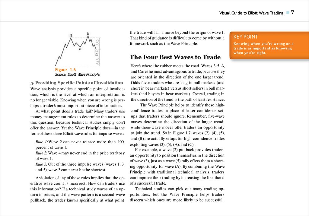
Also, corrections often retrace a Fibonacci percentage of the preceding wave. These Fibonacci-derived
regions allow traders to set profit-taking objectives
and identify areas where the next turn in prices will
likely occur (see Figures 1.5 and 1.6).
Figure 1.5
Source: Elliott Wave Principle.
27.
Visual Guide to Elliott Wave Tradingthe trade will fail: a move beyond the origin of wave 1.
That kind of guidance is difficult to come by without a
framework such as the Wave Principle.
The Four Best Waves to Trade
Figure 1.6
Source: Elliott Wave Principle.
5. Providing Speci c Points of Invalidation
Wave analysis provides a specific point of invalidation, which is the level at which an interpretation is
no longer viable. Knowing when you are wrong is perhaps a trader’s most important piece of information.
At what point does a trade fail? Many traders use
money management rules to determine the answer to
this question, because technical studies simply don’t
offer the answer. Yet the Wave Principle does—in the
form of these three Elliott wave rules for impulse waves:
Rule 1: Wave 2 can never retrace more than 100
percent of wave 1.
Rule 2: Wave 4 may never end in the price territory
of wave 1.
Rule 3: Out of the three impulse waves (waves 1, 3,
and 5), wave 3 can never be the shortest.
A violation of any of these rules implies that the operative wave count is incorrect. How can traders use
this information? If a technical study warns of an upturn in prices, and the wave pattern is a second-wave
pullback, the trader knows specifically at what point
Here’s where the rubber meets the road. Waves 3, 5, A,
and Care the most advantageous to trade, because they
are oriented in the direction of the one larger trend.
Odds favor traders who are long in bull markets (and
short in bear markets) versus short sellers in bull markets (and buyers in bear markets). Overall, trading in
the direction of the trend is the path of least resistance.
The Wave Principle helps to identify these highconfidence trades in place of lesser-confidence setups that traders should ignore. Remember, five-wave
moves determine the direction of the larger trend,
while three-wave moves offer traders an opportunity
to join the trend. So in Figure 1.7, waves (2), (4), (5),
and (B) are actually setups for high-confidence trades
exploiting waves (3), (5), (A), and (C).
For example, a wave (2) pullback provides traders
an opportunity to position themselves in the direction
of wave (3), just as a wave (5) rally offers them a shorting opportunity for wave (A). By combining the Wave
Principle with traditional technical analysis, traders
can improve their trading by increasing the likelihood
of a successful trade.
Technical studies can pick out many trading opportunities, but the Wave Principle helps traders
discern which ones are more likely to be successful.
■7
KEY POINT
Knowing when you’re wrong on a
trade is as important as knowing
when you’re right.
28.
8■
CHAPTER 1 The Anatomy of Elliott Wave Trading
Figure 1.7
This is because the Wave Principle is the framework
that provides history and context, current information, and a peek at the future.
Elliott Wave Trade Setups
This next chart (see Figure 1.7) shows bullish and bearish versions of trade setups. In each, waves (2), (4), (5),
and (B) are trade setups that introduce the four primary Elliott-based trading opportunities. These corrective
waves offer the trader an opportunity to rejoin the
larger trend. In such trend trading, a trader buys pullbacks in uptrends and sells bounces in downtrends.
When to Trade Corrections
Corrective waves offer less desirable trading opportunities because of their potential complexity. Impulse waves
are trend-defining price moves in which prices typically
travel far. Conversely, corrective wave patterns fluctuate more and can unfold slowly while taking a variety
of shapes, such as a zigzag, flat, expanded flat, triangle,
double zigzag, or combination. Corrections generally
move sideways and are often erratic, time-consuming,
and deceptive. Thus, it is emotionally exhausting to trade
corrections, and the odds of executing a successful trade
during this type of price action are low.
29.
Visual Guide to Elliott Wave TradingEven though I view corrective waves and patterns
as providing low-confidence trade setups, there are
times when I would consider trading them—but it depends on the potential duration of the correction. If I
count five waves up, for example, on a 15-minute price
chart of Crude Oil, I do not consider waves 2 or 4 to be
viable trading opportunities. I prefer, instead, to wait
for waves 2 and 4 to terminate before entering a position. Let’s say, though, that we have a market that has
also formed an impulse wave, but it has taken weeks
or months to do so. In this instance, waves 2 and 4
would form over many weeks and might offer traders
many short-term trading opportunities.
that a particular market is topping—and appropriate
price action does indeed corroborate this belief—then
the trader is more likely to execute a successful trade.
Guidelines for Trading Speci c
Elliott Wave Patterns
Although that guideline may sound complicated,
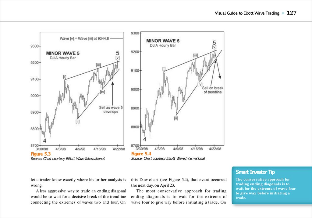
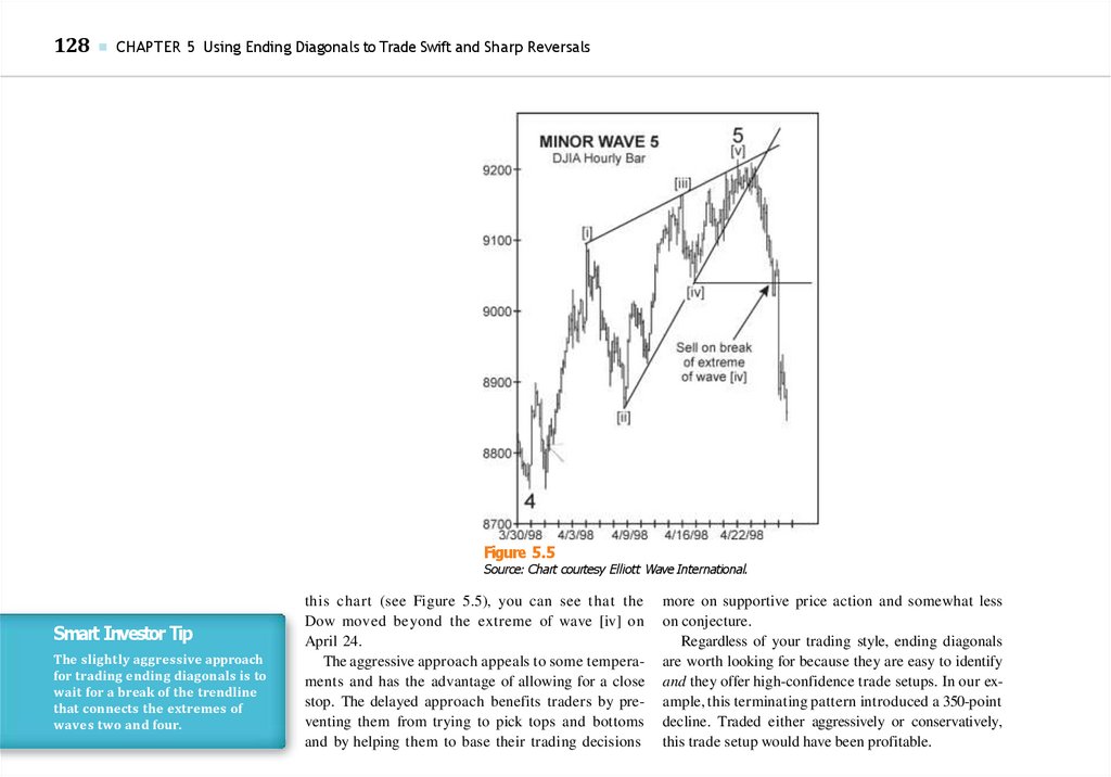
it’s easy to follow in real trading. The trading technique is to enter on a break below the extreme of
wave (iv) of 5 (see Figure 1.8). Doing so prevents top
picking and requires the market to take out a prior
swing low to act as initial evidence that the impulse
wave is indeed finished. Set the initial protective stop
at the extreme of the price move.
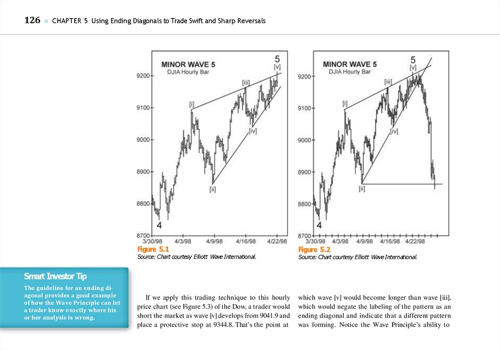
Before we review guidelines for trading specific Elliott
wave patterns, here is my most important analytical and trading rule: Let the market commit to you
before you commit to the market. In other words,
look for con rming price action. Just as it is unwise to
pull out in front of an oncoming car on the basis of its
turn signal alone, it is equally unwise to take a trade
without confirmation of a trend change.
The following guidelines incorporate this idea and
benefit the trader in two ways. First, waiting for confirming price action tends to decrease the number of
trades executed. One of the biggest mistakes traders
make is overtrading. Second, it focuses attention on
higher-confidence trade setups. If a trader believes
■9
Smart Investor Tip
Let the market commit to you
before you commit to the market.
Impulse Waves
Whenever an impulse wave is complete, the Elliott wave
guideline regarding the depth of corrective waves applies:
“[C]orrections, especially when they themselves
are fourth waves, tend to register their maximum
retracement within the span of travel of the previous
fourth wave of one lesser degree, most commonly
near the level of its terminus.”
—Elliott Wave Principle by Frost and Prechter
Ending Diagonal
The guidelines for entry and initial protective stops
for ending diagonals are similar to those for impulse
waves: Wait for a break of the extreme of wave 4 before
taking a position, and place the initial protective stop
at the extreme of the price move (see Figure 1.9).
Remember, these entry techniques demonstrate a
conservative approach that I think of as “ready, aim,
Smart Investor Tip
Waiting for con rming price
action allows traders to use an
evidence-based approach and to
focus their attention on highercon dence trade setups.
30.
10■
CHAPTER 1 The Anatomy of Elliott Wave Trading
Figure 1.8
Figure 1.9
31.
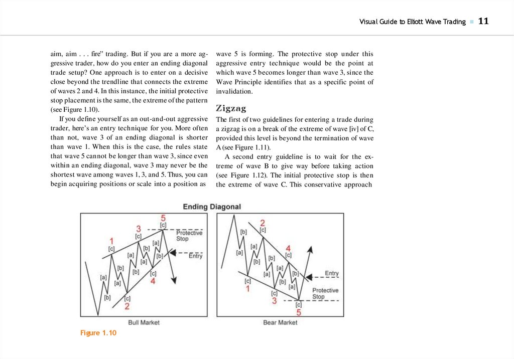
Visual Guide to Elliott Wave Trading ■aim, aim . . . fire” trading. But if you are a more aggressive trader, how do you enter an ending diagonal
trade setup? One approach is to enter on a decisive
close beyond the trendline that connects the extreme
of waves 2 and 4. In this instance, the initial protective
stop placement is the same, the extreme of the pattern
(see Figure 1.10).
If you define yourself as an out-and-out aggressive
trader, here’s an entry technique for you. More often
than not, wave 3 of an ending diagonal is shorter
than wave 1. When this is the case, the rules state
that wave 5 cannot be longer than wave 3, since even
within an ending diagonal, wave 3 may never be the
shortest wave among waves 1, 3, and 5. Thus, you can
begin acquiring positions or scale into a position as
Figure 1.10
wave 5 is forming. The protective stop under this
aggressive entry technique would be the point at
which wave 5 becomes longer than wave 3, since the
Wave Principle identifies that as a specific point of
invalidation.
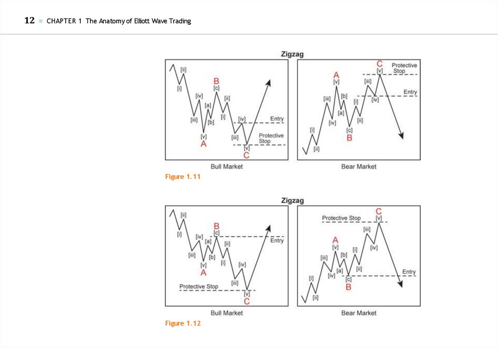
Zigzag
The first of two guidelines for entering a trade during
a zigzag is on a break of the extreme of wave [iv] of C,
provided this level is beyond the termination of wave
A (see Figure 1.11).
A second entry guideline is to wait for the extreme of wave B to give way before taking action
(see Figure 1.12). The initial protective stop is then
the extreme of wave C. This conservative approach
11
32.
12■
CHAPTER 1 The Anatomy of Elliott Wave Trading
Figure 1.11
Figure 1.12
33.
Visual Guide to Elliott Wave Trading ■prevents picking tops or bottoms without sufficient
evidence.
Ideally, traders will take these guidelines and
adapt them to their own specific trading style.
In fact, using a zigzag as an example, an even more
conservative trader could wait a bit longer before
entering and demand a five-wave move through
the extreme of wave B followed by a corrective wave
pattern.
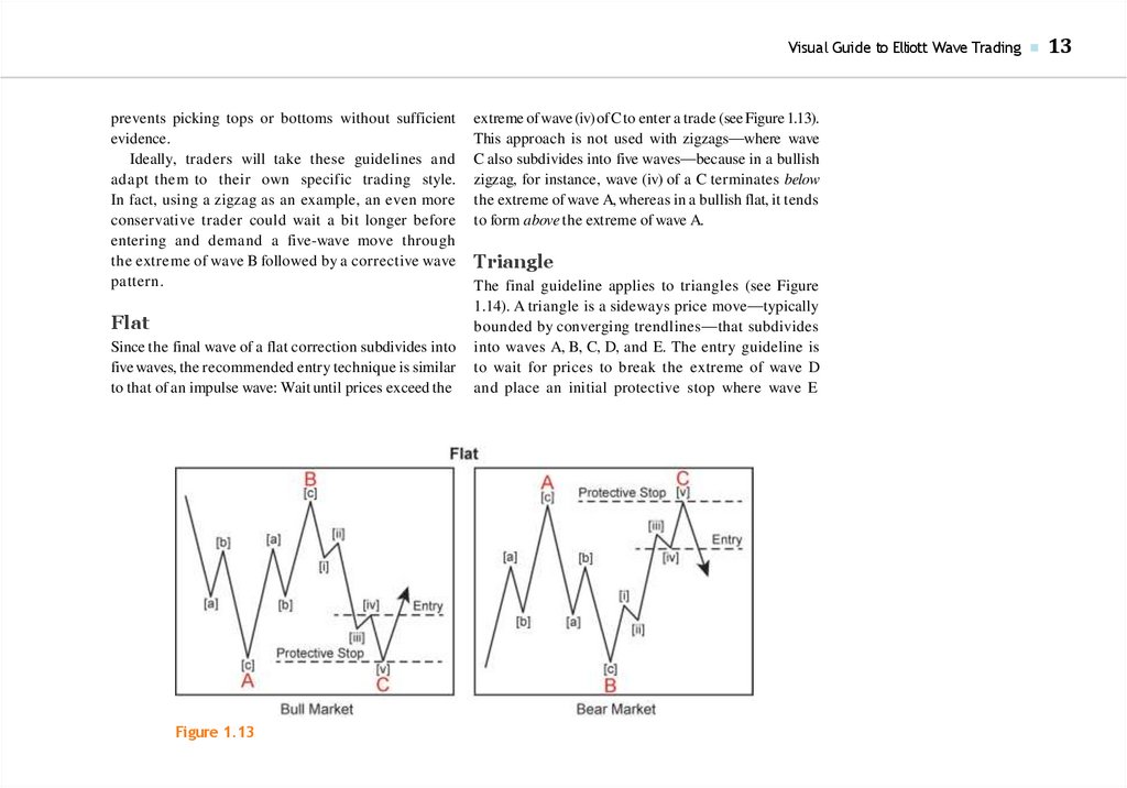
Flat
Since the final wave of a flat correction subdivides into
five waves, the recommended entry technique is similar
to that of an impulse wave: Wait until prices exceed the
Figure 1.13
extreme of wave (iv) of Cto enter a trade (see Figure 1.13).
This approach is not used with zigzags—where wave
C also subdivides into five waves—because in a bullish
zigzag, for instance, wave (iv) of a C terminates below
the extreme of wave A, whereas in a bullish flat, it tends
to form above the extreme of wave A.
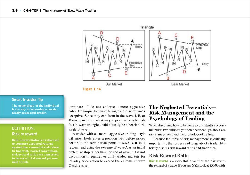
Triangle
The final guideline applies to triangles (see Figure
1.14). A triangle is a sideways price move—typically
bounded by converging trendlines—that subdivides
into waves A, B, C, D, and E. The entry guideline is
to wait for prices to break the extreme of wave D
and place an initial protective stop where wave E
13
34.
14■
CHAPTER 1 The Anatomy of Elliott Wave Trading
Figure 1.14
Smart Investor Tip
The psychology of the individual
is the key to becoming a consistently successful trader.
DEFINITION:
Risk to reward
Risk-Reward Ratio is a ratio used
to compare expected returns
against the amount of risk taken.
In line with market convention,
risk-reward ratios are expressed
in terms of total reward per one
unit of risk.
terminates. I do not endorse a more aggressive
entry technique because triangles are sometimes
deceptive: Since they can form in the wave 4, B, or
X wave positions, what may appear to be a bullish
fourth-wave triangle could actually be a bearish triangle B wave.
A trader with a more aggressive trading style
will most likely enter a position well before prices
penetrate the termination point of wave D. If so, I
recommend using the extreme of wave A as an initial
protective stop rather than the end of wave C. It is not
uncommon in equities or thinly traded markets for
intraday price action to exceed the extreme of wave
C and reverse.
The Neglected Essentials—
Risk Management and the
Psychology of Trading
When discussing how to become a consistently successful trader, two subjects you don’t hear enough about are
risk management and the psychology of trading.
Because the topic of risk management is critically
important to the success and longevity of a trader, let’s
briefly discuss risk-reward ratios and trade size.
Risk-Reward Ratio
Risk to reward is a ratio that quantifies the risk versus
the reward of a trade. If you buy XYZstock at $50.00 with
35.
Visual Guide to Elliott Wave Trading ■the expectation that it will appreciate to $51.00, your
expected reward is $1.00. If the protective stop on this
position is $49.00, the risk-reward ratio for this trade is
1:1—you’re risking $1.00 to make $1.00. If the protective
stop is $49.90, then the risk-reward ratio is 10:1.
Note: Even though it’s called a risk-reward ratio,
the ratio is conventionally stated with the reward
figure first. So, in this example, even though risk is
1 and the reward 10, the ratio is stated as 10:1, rather
than 1:10. This explains why a 3:1 risk-reward ratio is
desirable. It’s actually a reward-risk ratio.
Ahigh risk-reward ratio is desirable as a function of
probabilities. Let’s say that you’re right about the market 70 percent of the time, and the risk-reward ratio
on each of your trades is 1:1. Thus, out of 10 trades,
seven trades were closed with a $1.00 profit, while
three were exited with a $1.00 loss. The bottom line is
that you walked away with $4.00. What do you think
will happen if we increase the risk-reward ratio from
1:1 to 3:1 and decrease the probability of being right
from 70 percent to 40 percent? With this 3:1 ratio, for
the same $1.00 profit, four winning trades would net
$12.00. If we then subtract $6.00 in losing trades, we
walk away with a $6.00 profit.
This difference shows how important the riskreward ratio is—bydecreasing the probabilityof winning
trades from 70 percent to almost half (i.e., 40 percent)
while increasing the risk-reward ratio, you increase
profitability by 50 percent. A misconception about
trading is that a trader need be right only on the direction of the market to make money. This is not entirely
correct. As you’ve just seen, a trader can be right as little
as 40 percent of the time and still succeed, provided he
or she keeps an eye on the risk-reward ratio.
Smart Investor Tip
Trade Size
Trades that offer less than a
3:1 risk-reward ratio should be
avoided.
How large a position should a trader take? The risk
on a single trade should never exceed 1 to 3 percent
of the total portfolio size. Retail traders tend to balk
at these small percentages, while professional traders embrace them. Thus, at 1 percent, for every $5,000
a trader has in a trading account, he or she should
risk only $50 on each position. For example, a trader
with $10,000 in his account can take either two trades
where the risk is $50 apiece or one trade in which the
risk is $100. Many traders fail at trading because they
simply don’t have sufficient capital in their trading accounts to take the positions they want to take.
If you do have a small trading account, though,
you can overcome this challenge by trading small.
You can trade fewer contracts, trade e-mini contracts,
or even penny stocks. Bottom line, on your way to
becoming a consistently successful trader, you must
realize that longevity is key. If your risk on any given
position is small relative to your total capital, then
you can weather a losing streak. Conversely, if you risk
25 percent of your portfolio on each trade, after four
consecutive losers, you’re out of business.
The Psychology of Trading
While I consider risk management to be an essential component of successful trading, the true key is
psychology—that is, your individual psychology. Let’s
15
36.
16■
CHAPTER 1 The Anatomy of Elliott Wave Trading
Smart Investor Tip
Successful trading requires a
methodology and the discipline to
follow the methodology.
review a number of psychological factors that prevent
traders from becoming consistently successful: lack of
methodology, lack of discipline, unrealistic expectations, and lack of patience.
Whether you are a seasoned professional or just
thinking about opening your first trading account, it
is critically important to your success that you understand how your personal psychology affects your trading results.
Lack of Methodology
If you aim to be a consistently successful trader, then
you must have a defined trading methodology—a
simple, clear, and concise way of looking at markets.
In fact, having a method is so important that EWI
founder Robert Prechter put it at the top of his list
in his essay, “What a Trader Really Needs to Be Successful.” Guessing or going by gut instinct won’t work
over the long run. If you don’t have a defined trading
methodology, then you don’t have a way to know what
constitutes a buy or sell signal.
How do you overcome this problem? The answer
to this question is to write down your methodology.
Define in writing what your analytical tools are and,
more important, how you use them. It doesn’t matter
whether you use the Wave Principle, point and figure charts, stochastics, RSI, or a combination of all of
these. What does matter is that you actually make the
effort to define what constitutes a buy, a sell, your trailing stop, and instructions on exiting a position. The
best hint I can give you about defining your trading
methodology is this: If you can’t fit it on a 3" × 5" card,
it’s probably too complicated.
Lack of Discipline
Once you have clearly outlined and identified your
trading methodology, you must have the discipline
to follow the system. A lack of discipline while trading is the second common downfall of many aspiring
traders. If the way you view a price chart or evaluate a
potential trade setup today is different from how you
did it a month ago, then you either have not identified
your methodology or you lack the discipline to follow
the methodology you have identified. The formula for
success is to consistently apply a proven methodology.
Unrealistic Expectations
Nothing makes me angrier than those commercials
that say something like, “$5,000 properly positioned
in Natural Gas can give you returns of over $40,000.”
Advertisements like this are a disservice to the financial industry as a whole and end up costing uneducated investors a lot more than $5,000. In addition, they
help to create the psychologically sabotaging mindset of having unrealistic expectations.
Yes, it is possible to experience above-average returns trading your own account. However, it’s difficult
to do it without taking on above-average risk. So, what
is a realistic return to shoot for in your first year as a
trader—50 percent, 100 percent, 200 percent? Whoa,
let’s rein in those unrealistic expectations. In my opinion, the goal for every trader the first year out should
37.
Visual Guide to Elliott Wave Trading ■be not to lose money. In other words, shoot for a 0 percent return your first year. If you can manage that,
then in year two, try to beat the Dow or the S&P. These
goals may not be flashy, but they are realistic.
Lack of Patience
The fourth psychological pitfall that even experienced
traders encounter is a lack of patience. According to
Edwards and Magee in their seminal book, Technical
Analysis of Stock Trends, markets trend only about
30 percent of the time. This means that the other
70percent of the time, financial markets are not trending.
This small percentage may explain why I believe
that, for any given time frame, there are only two or
three really good trading opportunities. For example, if you’re a long-term trader, typically only two or
three compelling tradable moves in a market present
themselves during any given year. Similarly, if you are
a short-term trader, only two or three high-quality
trade setups present themselves in a given week.
All too often, because trading is inherently exciting
(and anything involving money usually is exciting), it’s
easy to feel that you’re missing something if you’re not
in a trade. As a result, you start taking trade setups of
lesser and lesser quality and begin overtrading.
How do you overcome this lack of patience? Remind
yourself that every week there will be another “trade of
the year.” In other words, don’t worry about missing an
opportunity today, because there will be another one
tomorrow, next week and next month . . . I promise.
For More Information
Learn more at your exclusive Reader Resources site.
You will find a free online edition of Elliott Wave
Principle by Frost and Prechter, plus lessons on Elliott
wave analysis, how to trade specific patterns, and how
to use Fibonacci and other technical indicators to increase your confidence as you apply the Wave Principle in real time. Go to: www.elliottwave.com/wave/
ReaderResources.
17
Smart Investor Tip
Stick with realistic expectations.
For instance, the goal for every
trader the rst year should be not
to lose money. In other words,
shoot for a 0 percent return during your rst year.
38.
18■
CHAPTER 1 The Anatomy of Elliott Wave Trading
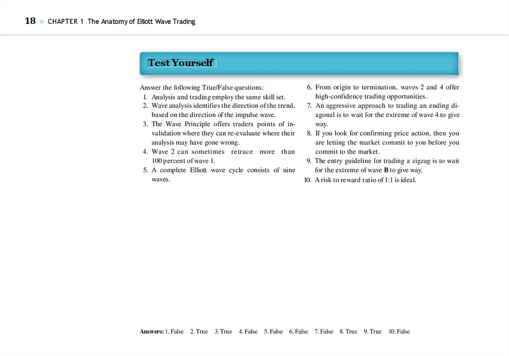
Test Yourself
Answer the following True/False questions:
1. Analysis and trading employ the same skill set.
2. Wave analysis identifies the direction of the trend,
based on the direction of the impulse wave.
3. The Wave Principle offers traders points of invalidation where they can re-evaluate where their
analysis may have gone wrong.
4. Wave 2 can sometimes retrace more than
100 percent of wave 1.
5. A complete Elliott wave cycle consists of nine
waves.
Answers: 1. False 2. True
3. True
4. False 5. False
6. From origin to termination, waves 2 and 4 offer
high-confidence trading opportunities.
7. An aggressive approach to trading an ending diagonal is to wait for the extreme of wave 4 to give
way.
8. If you look for confirming price action, then you
are letting the market commit to you before you
commit to the market.
9. The entry guideline for trading a zigzag is to wait
for the extreme of wave B to give way.
10. A risk to reward ratio of 1:1 is ideal.
6. False
7. False
8. True
9. True
10. False
39.
PAR TTrading Examples
40.
41.
CH AP TE RHow Zigzags and Flats Set Up a
Trade for the Next Impulse Wave
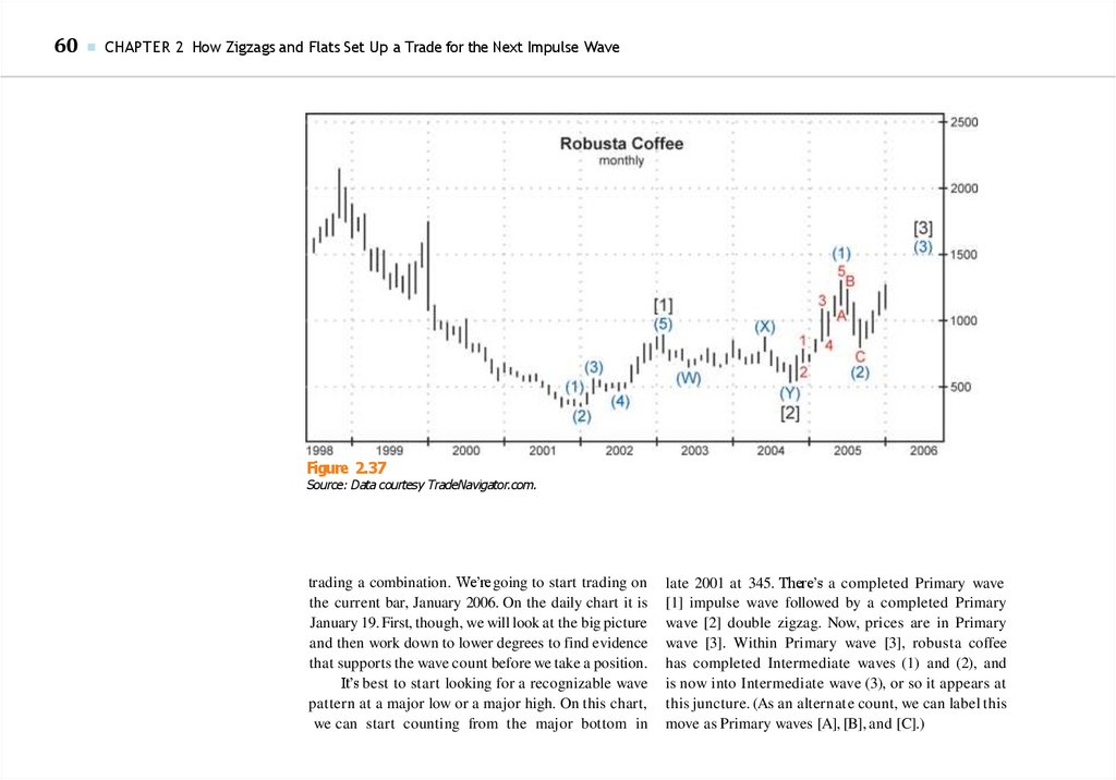
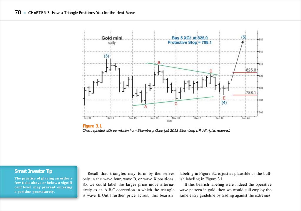
T
he three essential parts of a trade are analyzing
price charts, formulating a trading plan, and managing the trade.
Trading a Zigzag in
Caterpillar (CAT)
In Caterpillar (CAT), we’ll examine each component to better understand why CAT offered a highconfidence trade setup.
1. Analyzing the Price Charts
When it comes to trade setups, it doesn’t get much
easier than the price chart of CAT from April and May
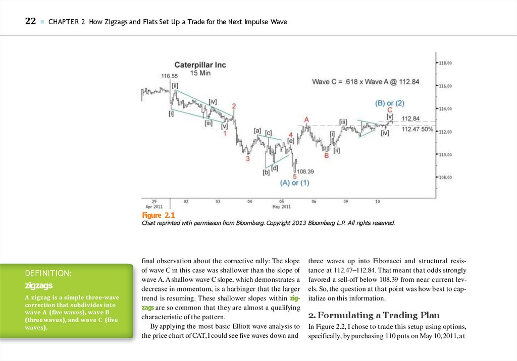
2011. As you can see in Figure 2.1, prices fell in five
waves from 116.55 to 108.39. This wave pattern was significant because impulse waves identify the direction
of the larger trend. Thus, this five-wave decline in CAT
implied further selling to come that would take prices
below 108.39 in either wave (C) or wave (3).
The subsequent rally in CAT that developed in
three waves supported this analysis. Countertrend
price action typically consists of three waves, so I
knew to expect another move down in CAT. Moreover, the three-wave advance in CAT traveled to
112.47 to retrace 50 percent of the previous sell-off.
That 50 percent is a common retracement for corrective waves. Also nearby was 112.84, the price level
at which wave C equaled a .618 multiple of wave A,
which is a common Fibonacci relationship between
waves C and A of corrective wave patterns.
The only question at this point was whether the
move up from 108.39 should be labeled as wave (B)
or wave (2). From a short-term trading perspective,
this question was academic because, either way, the
trade objective was a price move just under 108.39. A
KEY POINT
Impulse waves identify the
direction of the larger trend.
KEY POINT
Countertrend price action typically consists of three waves.
21
42.
22■
CHAPTER 2 How Zigzags and Flats Set Up a Trade for the Next Impulse Wave
Figure 2.1
Chart reprinted with permission from Bloomberg. Copyright 2013 Bloomberg L.P. All rights reserved.
DEFINITION:
zigzags
A zigzag is a simple three-wave
correction that subdivides into
wave A ( ve waves), wave B
(three waves), and wave C ( ve
waves).
final observation about the corrective rally: The slope
of wave C in this case was shallower than the slope of
wave A. Ashallow wave C slope, which demonstrates a
decrease in momentum, is a harbinger that the larger
trend is resuming. These shallower slopes within zigzags are so common that they are almost a qualifying
characteristic of the pattern.
By applying the most basic Elliott wave analysis to
the price chart of CAT,I could see five waves down and
three waves up into Fibonacci and structural resistance at 112.47–112.84. That meant that odds strongly
favored a sell-off below 108.39 from near current levels. So, the question at that point was how best to capitalize on this information.
2. Formulating a Trading Plan
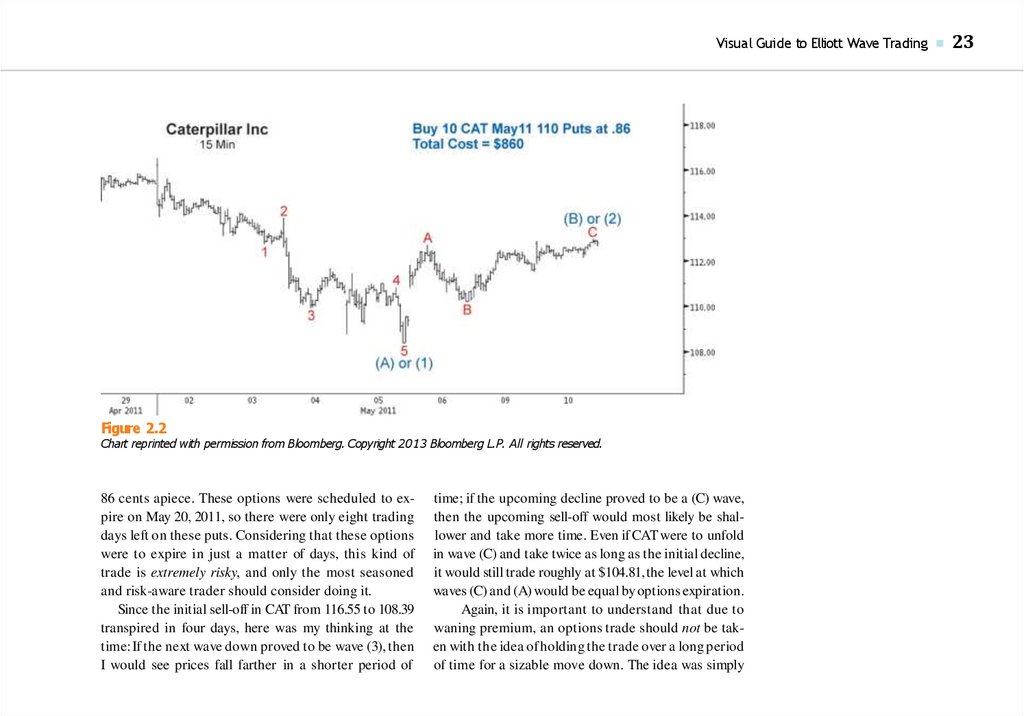
In Figure 2.2, I chose to trade this setup using options,
specifically, by purchasing 110 puts on May 10, 2011,at
43.
Visual Guide to Elliott Wave Trading ■Figure 2.2
Chart reprinted with permission from Bloomberg. Copyright 2013 Bloomberg L.P. All rights reserved.
86 cents apiece. These options were scheduled to expire on May 20, 2011, so there were only eight trading
days left on these puts. Considering that these options
were to expire in just a matter of days, this kind of
trade is extremely risky, and only the most seasoned
and risk-aware trader should consider doing it.
Since the initial sell-off in CAT from 116.55 to 108.39
transpired in four days, here was my thinking at the
time: If the next wave down proved to be wave (3), then
I would see prices fall farther in a shorter period of
time; if the upcoming decline proved to be a (C) wave,
then the upcoming sell-off would most likely be shallower and take more time. Even if CAT were to unfold
in wave (C) and take twice as long as the initial decline,
it would still trade roughly at $104.81,the level at which
waves (C) and (A) would be equal by options expiration.
Again, it is important to understand that due to
waning premium, an options trade should not be taken with the idea of holding the trade over a long period
of time for a sizable move down. The idea was simply
23
44.
24■
CHAPTER 2 How Zigzags and Flats Set Up a Trade for the Next Impulse Wave
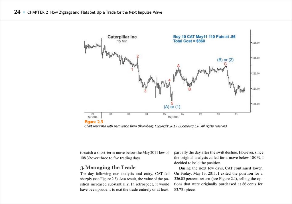
Figure 2.3
Chart reprinted with permission from Bloomberg. Copyright 2013 Bloomberg L.P. All rights reserved.
to catch a short-term move below the May 2011 low of
108.39 over three to five trading days.
3. Managing the Trade
The day following our analysis and entry, CAT fell
sharply (see Figure 2.3). As a result, the value of the position increased substantially. In retrospect, it would
have been prudent to exit the trade entirely or at least
partially the day after the swift decline. However, since
the original analysis called for a move below 108.39, I
decided to hold the position.
During the next few days, CAT continued lower.
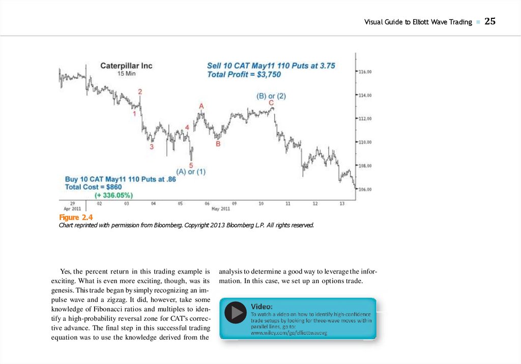
On Friday, May 13, 2011, I exited the position for a
336.05 percent return (see Figure 2.4), selling the options that were originally purchased at 86 cents for
$3.75 apiece.
45.
Visual Guide to Elliott Wave Trading ■Figure 2.4
Chart reprinted with permission from Bloomberg. Copyright 2013 Bloomberg L.P. All rights reserved.
Yes, the percent return in this trading example is
exciting. What is even more exciting, though, was its
genesis. This trade began by simply recognizing an impulse wave and a zigzag. It did, however, take some
knowledge of Fibonacci ratios and multiples to identify a high-probability reversal zone for CAT’s corrective advance. The final step in this successful trading
equation was to use the knowledge derived from the
analysis to determine a good way to leverage the information. In this case, we set up an options trade.
25
46.
26■
CHAPTER 2 How Zigzags and Flats Set Up a Trade for the Next Impulse Wave
KEY POINT
Always ask rst, “Do I see a wave
pattern I recognize?”
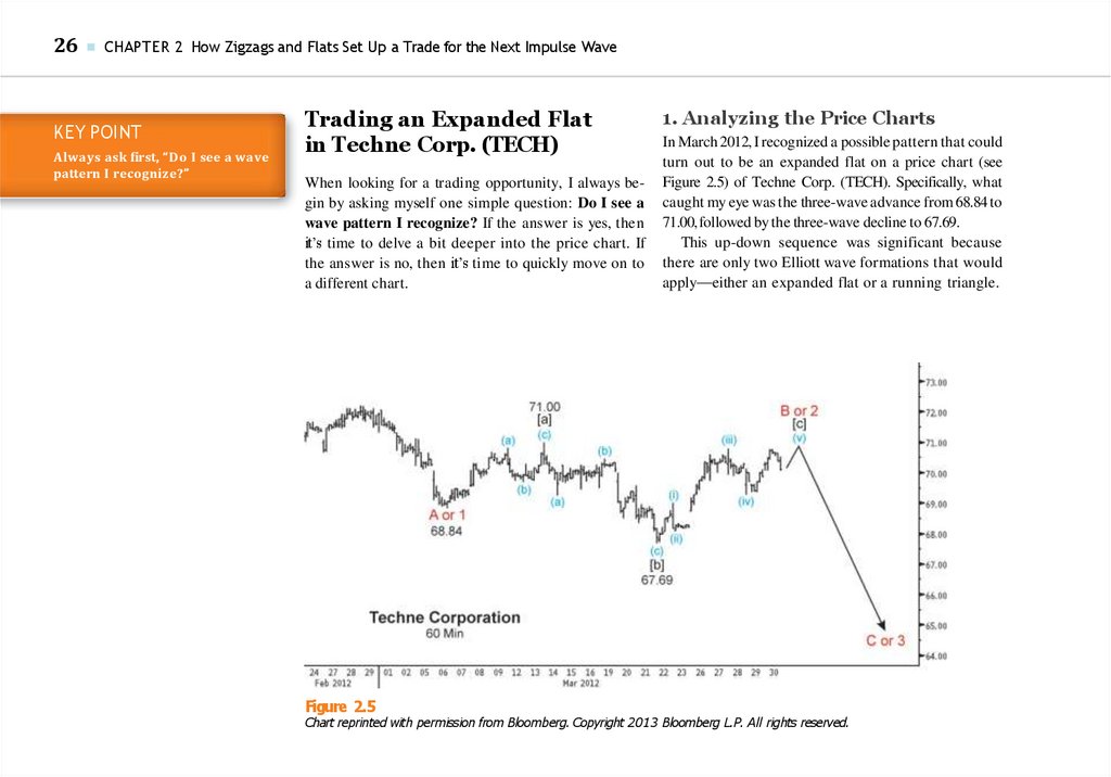
Trading an Expanded Flat
in Techne Corp. (TECH)
When looking for a trading opportunity, I always begin by asking myself one simple question: Do I see a
wave pattern I recognize? If the answer is yes, then
it’s time to delve a bit deeper into the price chart. If
the answer is no, then it’s time to quickly move on to
a different chart.
Figure 2.5
1. Analyzing the Price Charts
In March 2012, I recognized a possible pattern that could
turn out to be an expanded flat on a price chart (see
Figure 2.5) of Techne Corp. (TECH). Specifically, what
caught my eye was the three-wave advance from 68.84 to
71.00,followed by the three-wave decline to 67.69.
This up-down sequence was significant because
there are only two Elliott wave formations that would
apply—either an expanded flat or a running triangle.
Chart reprinted with permission from Bloomberg. Copyright 2013 Bloomberg L.P. All rights reserved.
47.
Visual Guide to Elliott Wave Trading ■Considering that the subsequent advance already had
four of the required five waves to complete an impulse
wave, odds strongly favored an expanded flat as the operative wave pattern in TECH.
2. Formulating a Trading Plan
Working with the hypothesis that an expanded flat
was forming in TECH, I put together my trading
Figure 2.6
plan, which was to sell 100 shares of TECH on a
move below the extreme of wave (iv) at 69.28 (see
Figure 2.6). As mentioned in Chapter 1, the guideline for entering a trade when the operative pattern
is a flat is to enter when prices move through the
extreme of wave four of C. This conservative approach should help prevent you from trying to pick
tops or bottoms.
Chart reprinted with permission from Bloomberg. Copyright 2013 Bloomberg L.P. All rights reserved.
27
DEFINITION:
expanded flat
An expanded at is a simple
three-wave correction that subdivides into wave A (three waves),
wave B (three waves), and wave
C ( ve waves), with wave B ending beyond the starting point of
wave A.
48.
28■
CHAPTER 2 How Zigzags and Flats Set Up a Trade for the Next Impulse Wave
Figure 2.7
Chart reprinted with permission from Bloomberg. Copyright 2013 Bloomberg L.P. All rights reserved.
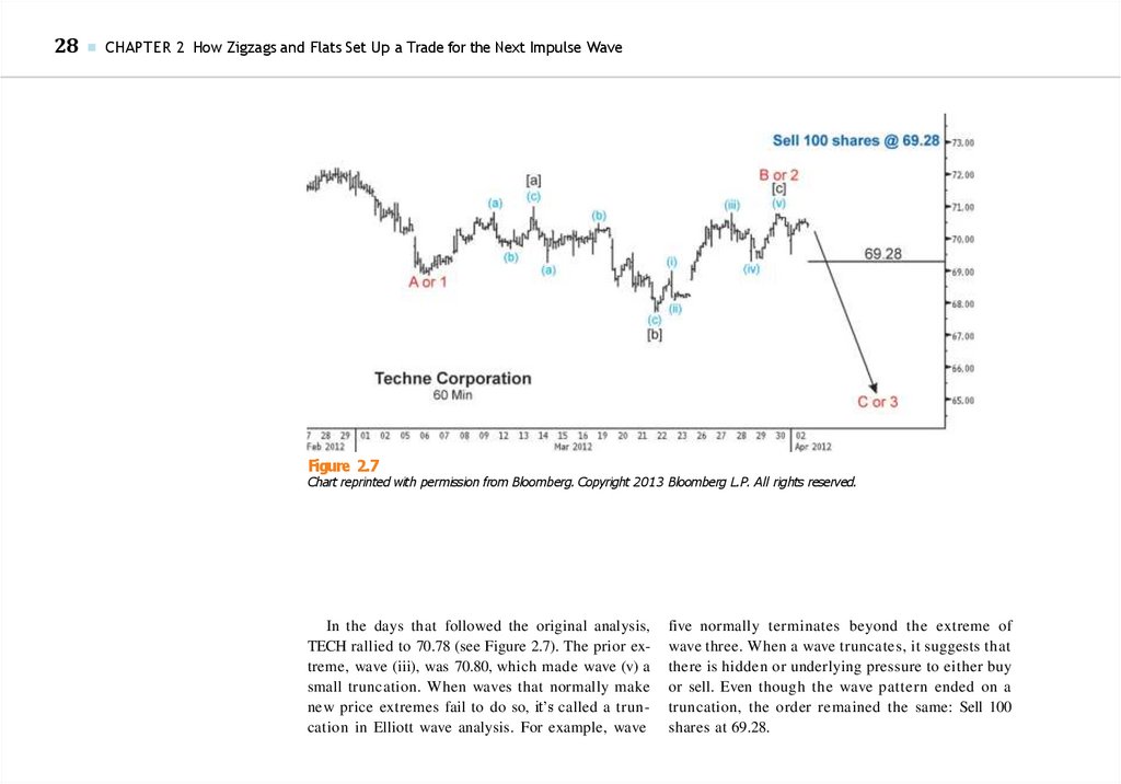
In the days that followed the original analysis,
TECH rallied to 70.78 (see Figure 2.7). The prior extreme, wave (iii), was 70.80, which made wave (v) a
small truncation. When waves that normally make
new price extremes fail to do so, it’s called a truncation in Elliott wave analysis. For example, wave
five normally terminates beyond the extreme of
wave three. When a wave truncates, it suggests that
there is hidden or underlying pressure to either buy
or sell. Even though the wave pattern ended on a
truncation, the order remained the same: Sell 100
shares at 69.28.
49.
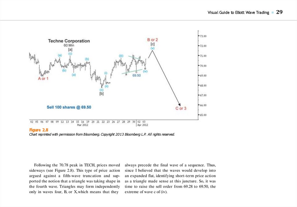
Visual Guide to Elliott Wave Trading ■Figure 2.8
Chart reprinted with permission from Bloomberg. Copyright 2013 Bloomberg L.P. All rights reserved.
Following the 70.78 peak in TECH, prices moved
sideways (see Figure 2.8). This type of price action
argued against a fifth-wave truncation and supported the notion that a triangle was taking shape in
the fourth wave. Triangles may form independently
only in waves four, B, or X, which means that they
always precede the final wave of a sequence. Thus,
since I believed that the waves would develop into
an expanded flat, identifying short-term price action
as a triangle made sense at this juncture. So, it was
time to raise the sell order from 69.28 to 69.50, the
extreme of wave c of (iv).
29
50.
30■
CHAPTER 2 How Zigzags and Flats Set Up a Trade for the Next Impulse Wave
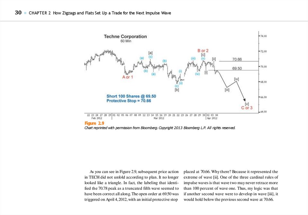
Figure 2.9
Chart reprinted with permission from Bloomberg. Copyright 2013 Bloomberg L.P. All rights reserved.
As you can see in Figure 2.9, subsequent price action
in TECH did not unfold according to plan. It no longer
looked like a triangle. In fact, the labeling that identified the 70.78 peak as a truncated fifth wave seemed to
have been correct all along. The open order at 69.50 was
triggered on April 4, 2012, with an initial protective stop
placed at 70.66. Why there? Because it represented the
extreme of wave [ii]. One of the three cardinal rules of
impulse waves is that wave two may never retrace more
than 100 percent of wave one. Thus, my logic was that
if another second wave were to develop in wave [iii], it
would hold below the previous second wave at 70.66.
51.
Visual Guide to Elliott Wave Trading ■31
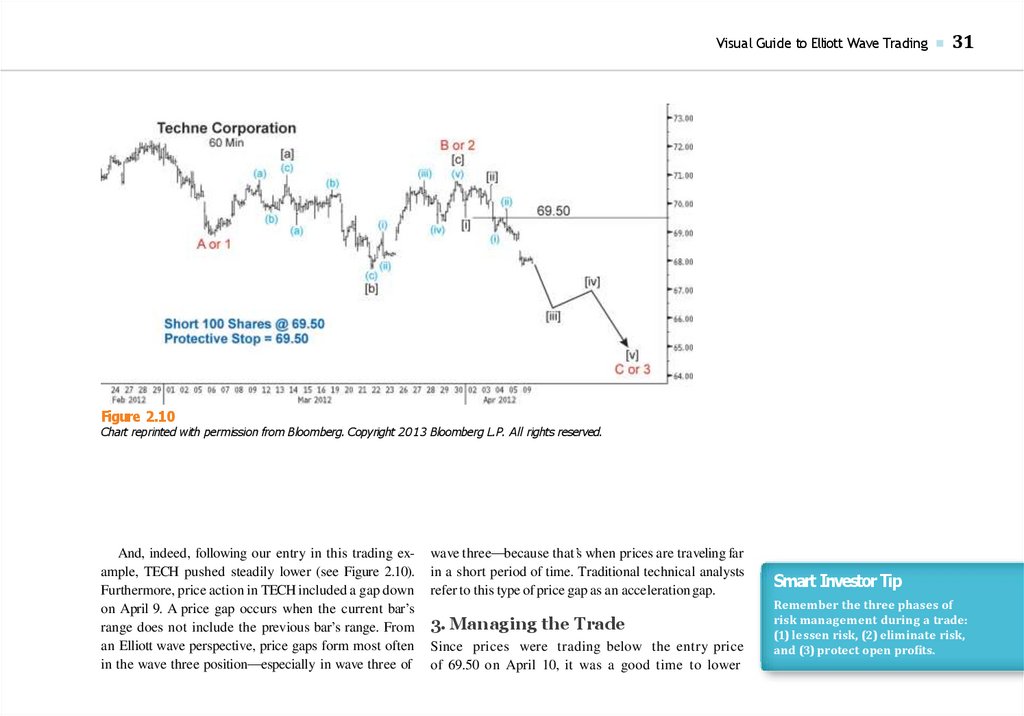
Figure 2.10
Chart reprinted with permission from Bloomberg. Copyright 2013 Bloomberg L.P. All rights reserved.
And, indeed, following our entry in this trading example, TECH pushed steadily lower (see Figure 2.10).
Furthermore, price action in TECH included a gap down
on April 9. A price gap occurs when the current bar’s
range does not include the previous bar’s range. From
an Elliott wave perspective, price gaps form most often
in the wave three position—especially in wave three of
wave three—because that’s when prices are traveling far
in a short period of time. Traditional technical analysts
refer to this type of price gap as an acceleration gap.
3. Managing the Trade
Since prices were trading below the entry price
of 69.50 on April 10, it was a good time to lower
Smart Investor Tip
Remember the three phases of
risk management during a trade:
(1) lessen risk, (2) eliminate risk,
and (3) protect open pro ts.
52.
32■
CHAPTER 2 How Zigzags and Flats Set Up a Trade for the Next Impulse Wave
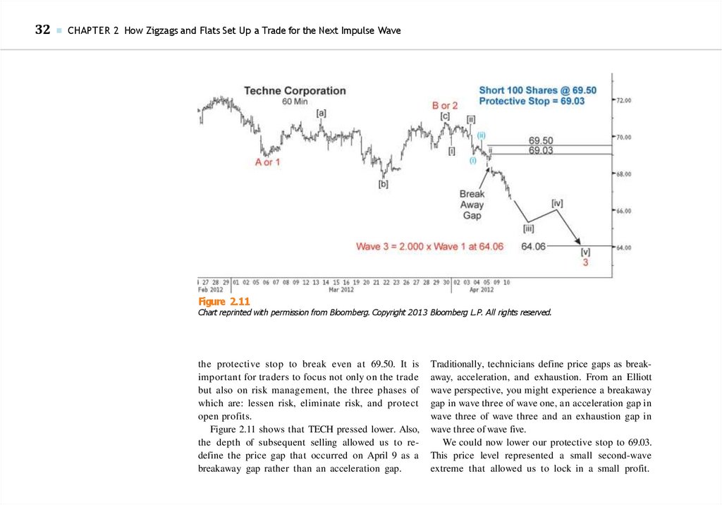
Figure 2.11
Chart reprinted with permission from Bloomberg. Copyright 2013 Bloomberg L.P. All rights reserved.
the protective stop to break even at 69.50. It is
important for traders to focus not only on the trade
but also on risk management, the three phases of
which are: lessen risk, eliminate risk, and protect
open profits.
Figure 2.11 shows that TECH pressed lower. Also,
the depth of subsequent selling allowed us to redefine the price gap that occurred on April 9 as a
breakaway gap rather than an acceleration gap.
Traditionally, technicians define price gaps as breakaway, acceleration, and exhaustion. From an Elliott
wave perspective, you might experience a breakaway
gap in wave three of wave one, an acceleration gap in
wave three of wave three and an exhaustion gap in
wave three of wave five.
We could now lower our protective stop to 69.03.
This price level represented a small second-wave
extreme that allowed us to lock in a small profit.
53.
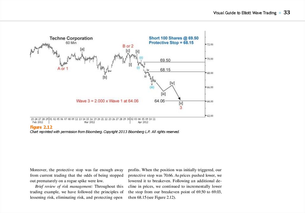
Visual Guide to Elliott Wave Trading ■Figure 2.12
Chart reprinted with permission from Bloomberg. Copyright 2013 Bloomberg L.P. All rights reserved.
Moreover, the protective stop was far enough away
from current trading that the odds of being stopped
out prematurely on a rogue spike were low.
Brief review of risk management: Throughout this
trading example, we have followed the principles of
lessening risk, eliminating risk, and protecting open
profits. When the position was initially triggered, our
protective stop was 70.66. As prices pushed lower, we
lowered it to breakeven. Following an additional decline in prices, we continued to incrementally lower
the stop from our breakeven point of 69.50 to 69.03,
then 68.15 (see Figure 2.12).
33
54.
34■
CHAPTER 2 How Zigzags and Flats Set Up a Trade for the Next Impulse Wave
Figure 2.13
Chart reprinted with permission from Bloomberg. Copyright 2013 Bloomberg L.P. All rights reserved.
Smart Investor Tip
While an impulsive decline is unfolding, prior swing highs make
suitable protective stops. From
an Elliott wave perspective, these
extremes tend to be second or
fourth waves.
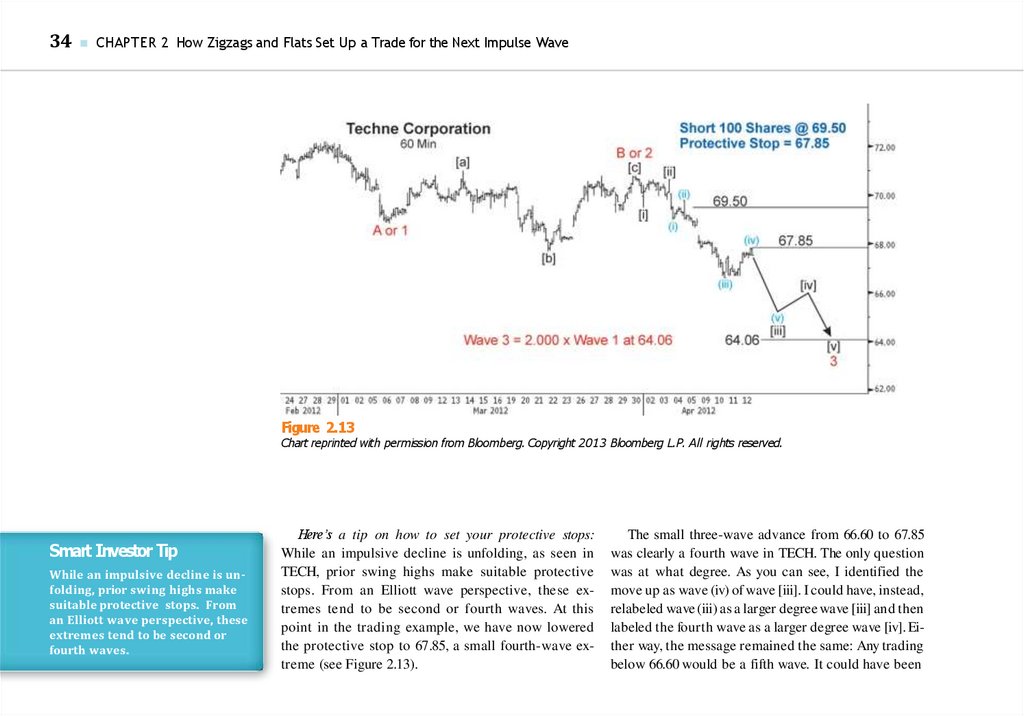
Here’s a tip on how to set your protective stops:
While an impulsive decline is unfolding, as seen in
TECH, prior swing highs make suitable protective
stops. From an Elliott wave perspective, these extremes tend to be second or fourth waves. At this
point in the trading example, we have now lowered
the protective stop to 67.85, a small fourth-wave extreme (see Figure 2.13).
The small three-wave advance from 66.60 to 67.85
was clearly a fourth wave in TECH. The only question
was at what degree. As you can see, I identified the
move up as wave (iv) of wave [iii]. I could have, instead,
relabeled wave (iii) as a larger degree wave [iii] and then
labeled the fourth wave as a larger degree wave [iv]. Either way, the message remained the same: Any trading
below 66.60 would be a fifth wave. It could have been
55.
Visual Guide to Elliott Wave Trading ■Figure 2.14
Chart reprinted with permission from Bloomberg. Copyright 2013 Bloomberg L.P. All rights reserved.
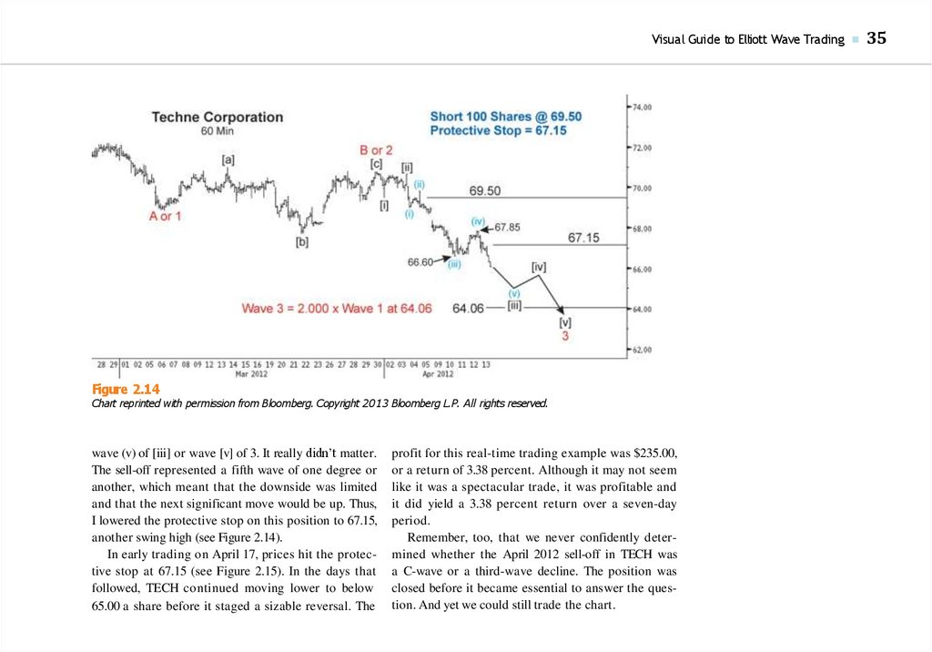
wave (v) of [iii] or wave [v] of 3. It really didn’t matter.
The sell-off represented a fifth wave of one degree or
another, which meant that the downside was limited
and that the next significant move would be up. Thus,
I lowered the protective stop on this position to 67.15,
another swing high (see Figure 2.14).
In early trading on April 17, prices hit the protective stop at 67.15 (see Figure 2.15). In the days that
followed, TECH continued moving lower to below
65.00 a share before it staged a sizable reversal. The
profit for this real-time trading example was $235.00,
or a return of 3.38 percent. Although it may not seem
like it was a spectacular trade, it was profitable and
it did yield a 3.38 percent return over a seven-day
period.
Remember, too, that we never confidently determined whether the April 2012 sell-off in TECH was
a C-wave or a third-wave decline. The position was
closed before it became essential to answer the question. And yet we could still trade the chart.
35
56.
36■
CHAPTER 2 How Zigzags and Flats Set Up a Trade for the Next Impulse Wave
Figure 2.15
Chart reprinted with permission from Bloomberg. Copyright 2013 Bloomberg L.P. All rights reserved.
Overall, this trade shows the beauty of the Wave
Principle and the incredible power of one very simple question: “Do I see a wave pattern I recognize?”
Because I could answer yes to this question, I was able
to formulate a trading plan that ultimately proved to
be profitable.
Might I have done a better job trading this position, perhaps by getting in earlier or exiting the
position when TECH fell below 65.00? Did I trail my
protective stops correctly or was I too aggressive or
too conservative? My simple answer remains true:
There is no right or wrong way to trade—only your
way of trading. Bottom line, this was a profitable
position that was vulnerable to a loss for only two
trading days before we could implement a breakeven stop.
57.
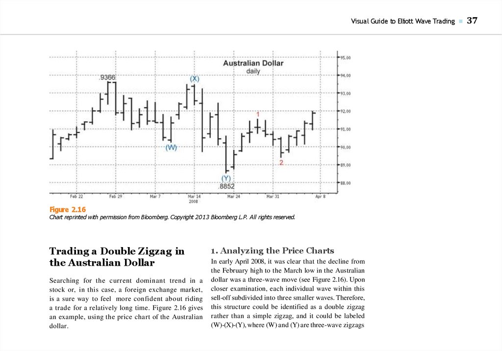
Visual Guide to Elliott Wave Trading ■Figure 2.16
Chart reprinted with permission from Bloomberg. Copyright 2013 Bloomberg L.P. All rights reserved.
Trading a Double Zigzag in
the Australian Dollar
Searching for the current dominant trend in a
stock or, in this case, a foreign exchange market,
is a sure way to feel more confident about riding
a trade for a relatively long time. Figure 2.16 gives
an example, using the price chart of the Australian
dollar.
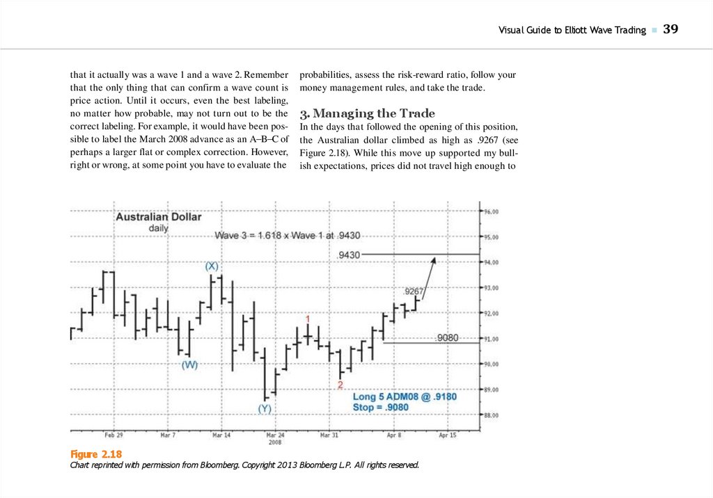
1. Analyzing the Price Charts
In early April 2008, it was clear that the decline from
the February high to the March low in the Australian
dollar was a three-wave move (see Figure 2.16). Upon
closer examination, each individual wave within this
sell-off subdivided into three smaller waves. Therefore,
this structure could be identified as a double zigzag
rather than a simple zigzag, and it could be labeled
(W)-(X)-(Y), where (W) and (Y) are three-wave zigzags
37
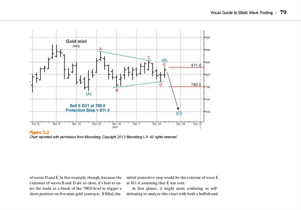
58.
38■
CHAPTER 2 How Zigzags and Flats Set Up a Trade for the Next Impulse Wave
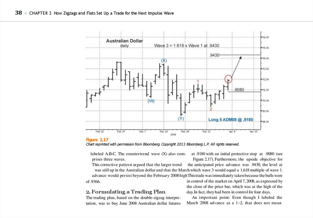
Figure 2.17
Chart reprinted with permission from Bloomberg. Copyright 2013 Bloomberg L.P. All rights reserved.
labeled A-B-C. The countertrend wave (X) also com- at .9180 with an initial protective stop at .9080 (see
prises three waves.
Figure 2.17). Furthermore, the upside objective for
This corrective pattern argued that the larger trend the anticipated price advance was .9430, the level at
was still up in the Australian dollar and that the March which wave 3 would equal a 1.618 multiple of wave 1.
advance would persist beyond the February 2008 highThistrade was immediately taken because the bulls were
in control of the market on April 7, 2008, as expressed by
of .9366.
the close of the price bar, which was at the high of the
day. In fact, they had been in control for four days.
2. Formulating a Trading Plan
An important point: Even though I labeled the
The trading plan, based on the double-zigzag interpreMarch
2008 advance as a 1–2, that does not mean
tation, was to buy June 2008 Australian dollar futures
59.
Visual Guide to Elliott Wave Trading ■that it actually was a wave 1 and a wave 2. Remember
that the only thing that can confirm a wave count is
price action. Until it occurs, even the best labeling,
no matter how probable, may not turn out to be the
correct labeling. For example, it would have been possible to label the March 2008 advance as an A–B–C of
perhaps a larger flat or complex correction. However,
right or wrong, at some point you have to evaluate the
Figure 2.18
probabilities, assess the risk-reward ratio, follow your
money management rules, and take the trade.
3. Managing the Trade
In the days that followed the opening of this position,
the Australian dollar climbed as high as .9267 (see
Figure 2.18). While this move up supported my bullish expectations, prices did not travel high enough to
Chart reprinted with permission from Bloomberg. Copyright 2013 Bloomberg L.P. All rights reserved.
39
60.
40■
CHAPTER 2 How Zigzags and Flats Set Up a Trade for the Next Impulse Wave
Figure 2.19
Chart reprinted with permission from Bloomberg. Copyright 2013 Bloomberg L.P. All rights reserved.
allow me to raise or tighten the protective stops. Thus,
the initial protective stop remained at .9080.
Then price action created what appeared to be
a small wave 3 peak at .9267 (see Figure 2.19). In the
days that followed, the Australian dollar fell 140 pips
to .9127. This decline of 1.51 percent in two days was
a decent-sized move, and it initially supported my
bearish interpretation of the March advance. But
what prevented me from adopting a bearish assessment on April 14, following the 140 pip sell-off, was the
close of the daily price bar. It was .9166, basis the June
contract.
By itself, this information seemed to be unimportant. But combined with the high and low of the
61.
Visual Guide to Elliott Wave Trading ■Figure 2.20
Chart reprinted with permission from Bloomberg. Copyright 2013 Bloomberg L.P. All rights reserved.
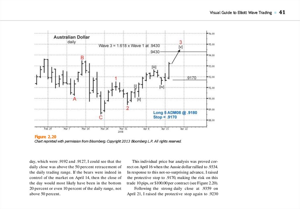
day, which were .9192 and .9127, I could see that the
daily close was above the 50 percent retracement of
the daily trading range. If the bears were indeed in
control of the market on April 14, then the close of
the day would most likely have been in the bottom
20 percent or even 10 percent of the daily range, not
above 50 percent.
This individual price bar analysis was proved correct on April 16 when the Aussie dollar rallied to .9334.
In response to this not-so-surprising advance, I raised
the protective stop to .9170, making the risk on this
trade 10 pips, or $100.00 per contract (see Figure 2.20).
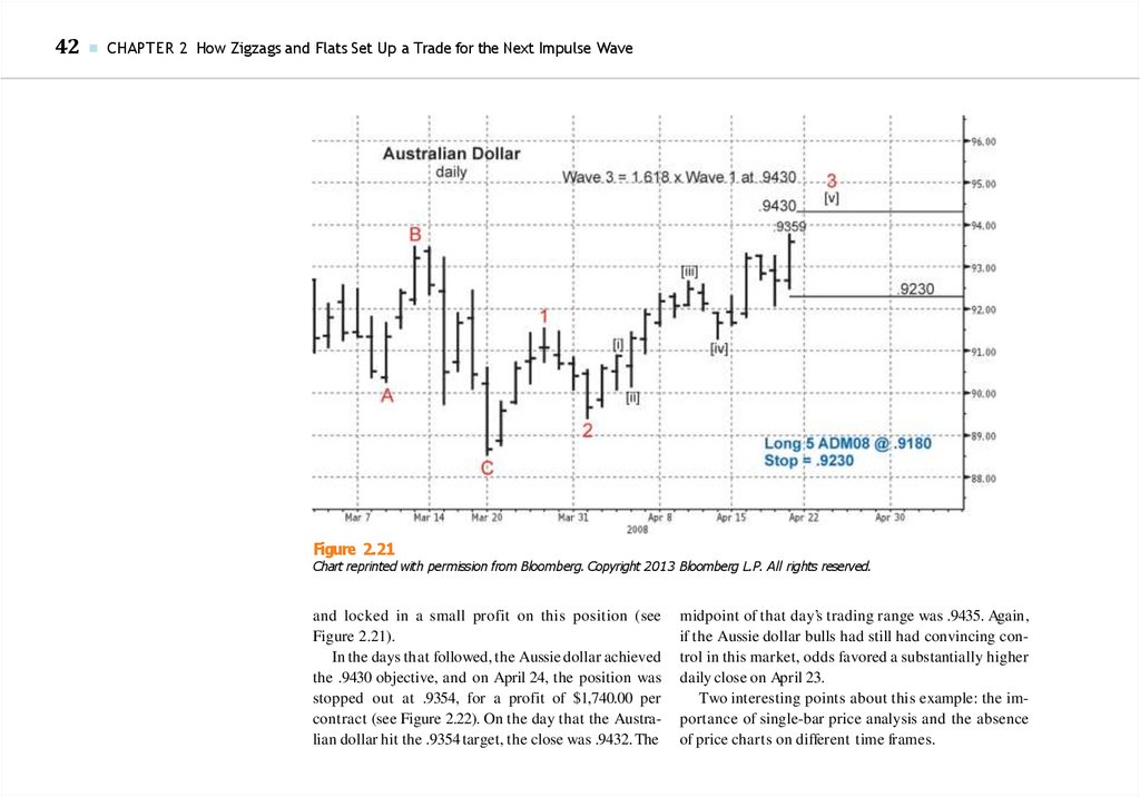
Following the strong daily close at .9359 on
April 21, I raised the protective stop again to .9230
41
62.
42■
CHAPTER 2 How Zigzags and Flats Set Up a Trade for the Next Impulse Wave
Figure 2.21
Chart reprinted with permission from Bloomberg. Copyright 2013 Bloomberg L.P. All rights reserved.
and locked in a small profit on this position (see
Figure 2.21).
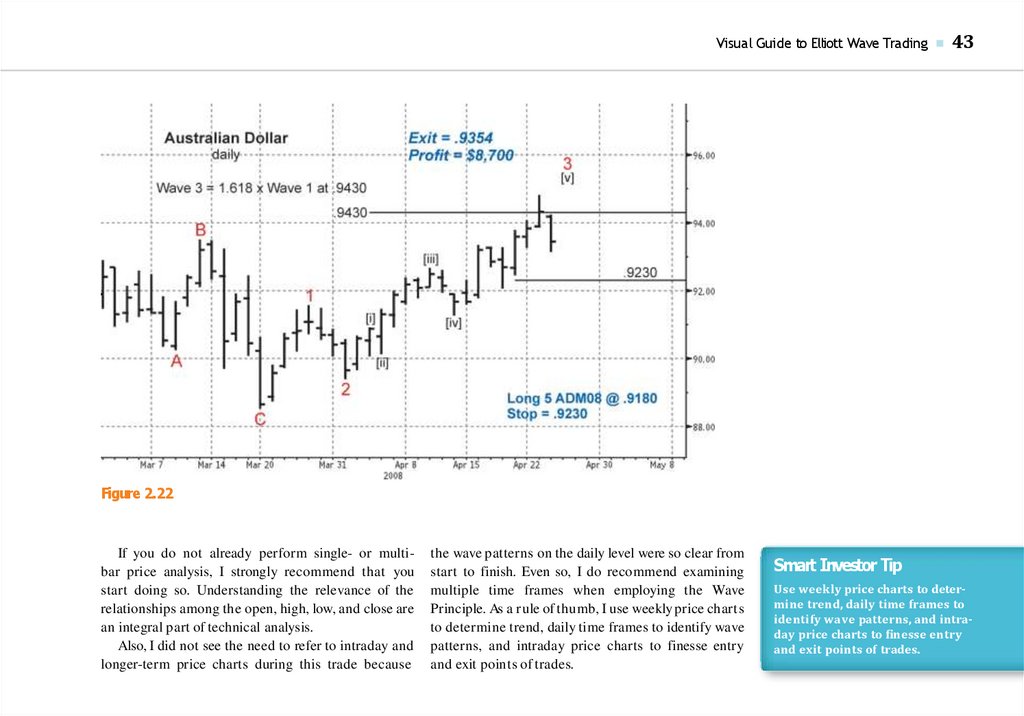
In the days that followed, the Aussie dollar achieved
the .9430 objective, and on April 24, the position was
stopped out at .9354, for a profit of $1,740.00 per
contract (see Figure 2.22). On the day that the Australian dollar hit the .9354 target, the close was .9432. The
midpoint of that day’s trading range was .9435. Again,
if the Aussie dollar bulls had still had convincing control in this market, odds favored a substantially higher
daily close on April 23.
Two interesting points about this example: the importance of single-bar price analysis and the absence
of price charts on different time frames.
63.
Visual Guide to Elliott Wave Trading ■43
Figure 2.22
If you do not already perform single- or multibar price analysis, I strongly recommend that you
start doing so. Understanding the relevance of the
relationships among the open, high, low, and close are
an integral part of technical analysis.
Also, I did not see the need to refer to intraday and
longer-term price charts during this trade because
the wave patterns on the daily level were so clear from
start to finish. Even so, I do recommend examining
multiple time frames when employing the Wave
Principle. As a rule of thumb, I use weekly price charts
to determine trend, daily time frames to identify wave
patterns, and intraday price charts to finesse entry
and exit points of trades.
Smart Investor Tip
Use weekly price charts to determine trend, daily time frames to
identify wave patterns, and intraday price charts to nesse entry
and exit points of trades.
64.
44■
CHAPTER 2 How Zigzags and Flats Set Up a Trade for the Next Impulse Wave
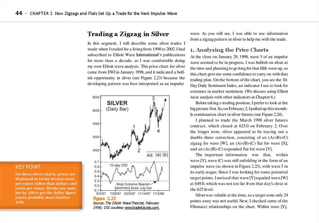
Trading a Zigzag in Silver
In this segment, I will describe some silver trades I
made when I traded for a living from 1998 to 2002. I had
subscribed to Elliott Wave International’s publications
for more than a decade, so I was comfortable doing
my own Elliott wave analysis. This price chart for silver
came from EWI in January 1998, and it indicated a bullish opportunity in silver (see Figure 2.23) because the
developing pattern was best interpreted as an impulse
KEY POINT
On these silver charts, prices are
displayed in terms of total cents
per ounce rather than dollars and
cents per ounce. Divide any number by 100 to get the dollar gure
you’re probably most familiar
with.
Figure 2.23
Source: The Elliott WaveTheorist, February
1998; DSI courtesy www.tradefutures.com.
wave. As you will see, I was able to use information
from a zigzag pattern in silver to help me with the trade.
1. Analyzing the Price Charts
At the close on January 29, 1998, wave 5 of an impulse
wave seemed to be in progress. I was bullish on silver at
the time and planning to go long for that fifth wave up, so
this chart gave me some confidence to carry on with that
trading plan. On the bottom of the chart, you see the 10Day Daily Sentiment Index, an indicator I use to look for
extremes in market sentiment. (We discuss using Elliott
wave analysis with other indicators in Chapter 6.)
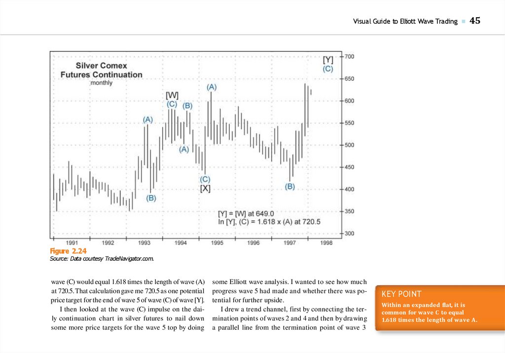
Before taking a trading position, I prefer to look at the
big picture first. So,on February 2,I pulled up this monthly continuation chart in silver futures (see Figure 2.24).
I planned to trade the March 1998 silver futures
contract, which closed at 625.0 on February 2. Over
the longer term, silver appeared to be tracing out a
double three correction, consisting of an (A)-(B)-(C)
zigzag for wave [W], an (A)-(B)-(C) flat for wave [X],
and an (A)-(B)-(C) expanded flat for wave [Y].
The important information was that, within
wave [Y], wave (C) was still unfolding in the form of an
impulse wave (as shown in Figure 2.23), with wave 5 in
its early stages. Since I was looking for some potential
target points, I noticed that wave [Y] equaled wave [W]
at 649.0, which was not too far from that day’s close at
the 625 level.
Silver was volatile at the time, so a target zone only 24
points away was not useful. Next, I checked some of the
Fibonacci relationships on the chart. Within wave [Y],
65.
Visual Guide to Elliott Wave Trading ■45
Figure 2.24
Source: Data courtesy TradeNavigator.com.
wave (C) would equal 1.618 times the length of wave (A)
at 720.5.That calculation gave me 720.5 as one potential
price target for the end of wave 5 of wave (C) of wave [Y].
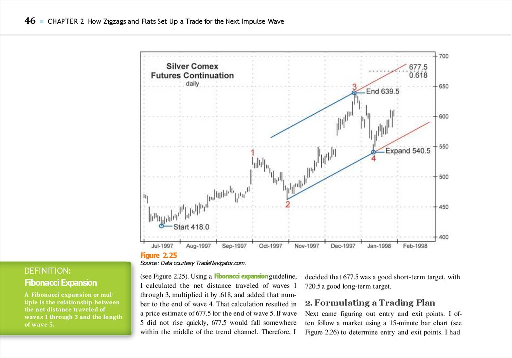
I then looked at the wave (C) impulse on the daily continuation chart in silver futures to nail down
some more price targets for the wave 5 top by doing
some Elliott wave analysis. I wanted to see how much
progress wave 5 had made and whether there was potential for further upside.
I drew a trend channel, first by connecting the termination points of waves 2 and 4 and then by drawing
a parallel line from the termination point of wave 3
KEY POINT
Within an expanded at, it is
common for wave C to equal
1.618 times the length of wave A.
66.
46■
CHAPTER 2 How Zigzags and Flats Set Up a Trade for the Next Impulse Wave
Figure 2.25
DEFINITION:
Fibonacci Expansion
A Fibonacci expansion or multiple is the relationship between
the net distance traveled of
waves 1 through 3 and the length
of wave 5.
Source: Data courtesy TradeNavigator.com.
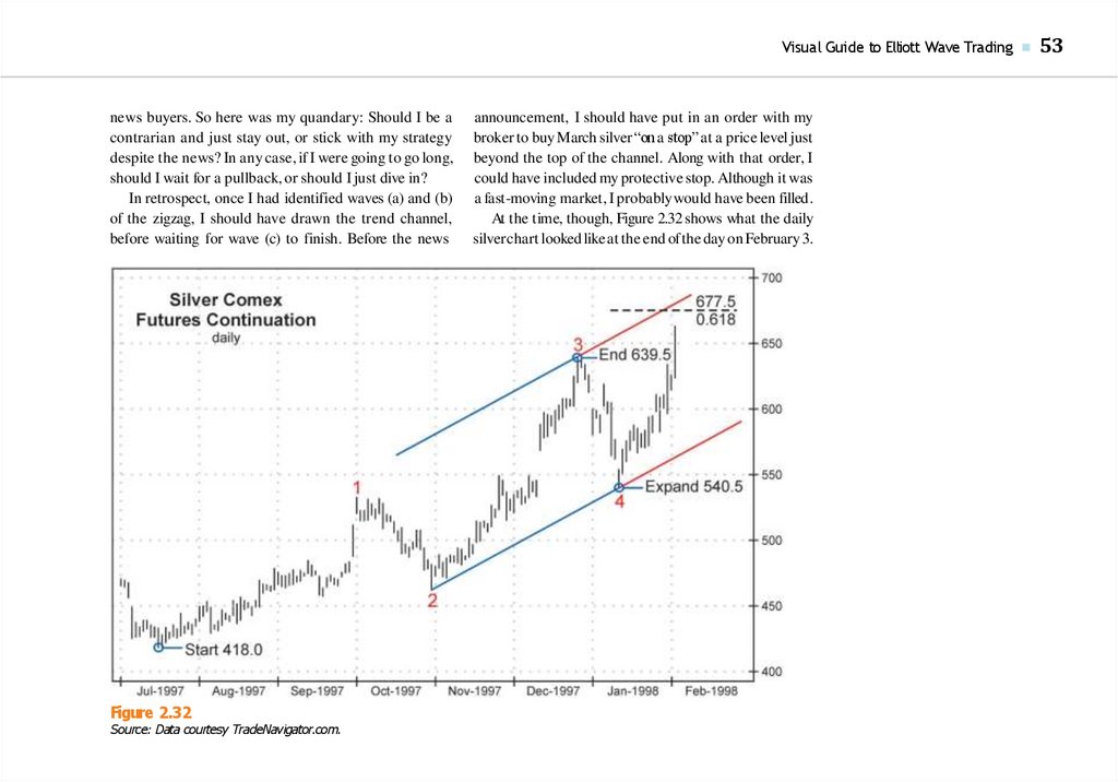
(see Figure 2.25). Using a Fibonacci expansion guideline,
I calculated the net distance traveled of waves 1
through 3, multiplied it by .618, and added that number to the end of wave 4. That calculation resulted in
a price estimate of 677.5 for the end of wave 5. If wave
5 did not rise quickly, 677.5 would fall somewhere
within the middle of the trend channel. Therefore, I
decided that 677.5 was a good short-term target, with
720.5 a good long-term target.
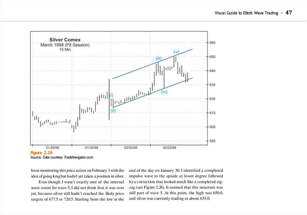
2. Formulating a Trading Plan
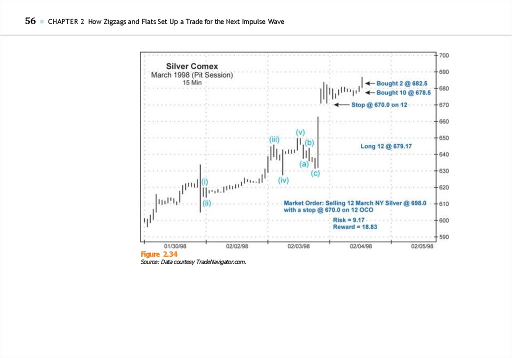
Next came figuring out entry and exit points. I often follow a market using a 15-minute bar chart (see
Figure 2.26) to determine entry and exit points. I had
67.
Visual Guide to Elliott Wave Trading ■Figure 2.26
Source: Data courtesy TradeNavigator.com.
been monitoring this price action on February 3 with the
idea of going long but hadn’t yet taken a position in silver.
Even though I wasn’t exactly sure of the internal
wave count for wave 5, I did not think that it was over
yet, because silver still hadn’t reached the likely price
targets of 677.5 or 720.5. Starting from the low at the
end of the day on January 30, I identified a completed
impulse wave to the upside at lower degree followed
by a correction that looked much like a completed zigzag (see Figure 2.26). It seemed that this structure was
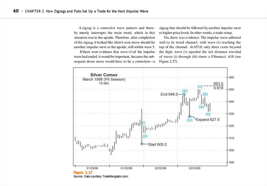
still part of wave 5. At this point, the high was 650.0,
and silver was currently trading at about 635.0.
47
68.
48■
CHAPTER 2 How Zigzags and Flats Set Up a Trade for the Next Impulse Wave
A zigzag is a corrective wave pattern and thereby merely interrupts the main trend, which in this
situation was to the upside. Therefore, after completion
of the zigzag, it looked like silver’s next move should be
another impulse wave to the upside, still within wave 5.
If there were evidence that wave (v) of the impulse
wave had ended, it would be important, because the subsequent down move would have to be a correction—a
Figure 2.27
Source: Data courtesy TradeNavigator.com.
zigzag that should be followed by another impulse wave
to higher price levels. In other words, a trade setup.
Yes, there was evidence. The impulse wave adhered
well to its trend channel, with wave (v) reaching the
top of the channel. At 653.0, only three cents beyond
the high, wave (v) equaled the net distance traveled
of waves (i) through (iii) times a Fibonacci .618 (see
Figure 2.27).
69.
Visual Guide to Elliott Wave Trading ■Figure 2.28
DEFINITION:
Golden Section
Source: Data courtesy TradeNavigator.com.
There was more supporting evidence: As shown in
the next chart (see Figure 2.28), if wave (v) had ended at 650.0, then the end of wave (iv) would have divided the entire price range of the impulse wave into
two equal parts, which is a Fibonacci relationship in
49
completed impulse waves called a Fibonacci price divider. More commonly, fourth waves divide the entire
price range into the Golden Section.
Other evidence also supported the idea that the
zigzag on the 15-minute chart was complete. As
The beginning or end of wave 4
will often divide an impulse
wave into the Golden Section
(.618 and .382) or two equal parts.
This relationship is called a Fibonacci price divider.
70.
50■
CHAPTER 2 How Zigzags and Flats Set Up a Trade for the Next Impulse Wave
Figure 2.29
Source: Data courtesy TradeNavigator.com.
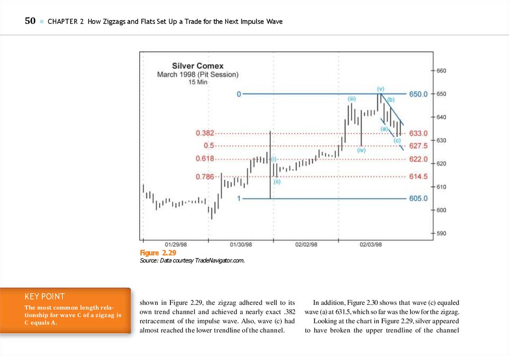
KEY POINT
The most common length relationship for wave C of a zigzag is
C equals A.
shown in Figure 2.29, the zigzag adhered well to its
own trend channel and achieved a nearly exact .382
retracement of the impulse wave. Also, wave (c) had
almost reached the lower trendline of the channel.
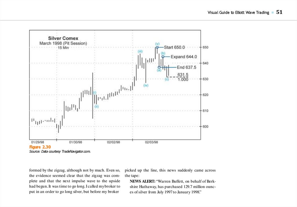
In addition, Figure 2.30 shows that wave (c) equaled
wave (a) at 631.5,which so far was the low for the zigzag.
Looking at the chart in Figure 2.29, silver appeared
to have broken the upper trendline of the channel
71.
Visual Guide to Elliott Wave Trading ■Figure 2.30
Source: Data courtesy TradeNavigator.com.
formed by the zigzag, although not by much. Even so,
the evidence seemed clear that the zigzag was complete and that the next impulse wave to the upside
had begun. It was time to go long. I called my broker to
put in an order to go long silver, but before my broker
picked up the line, this news suddenly came across
the tape:
NEWS ALERT: “Warren Buffett, on behalf of Berkshire Hathaway, has purchased 129.7 million ounces of silver from July 1997 to January 1998.”
51
72.
52■
CHAPTER 2 How Zigzags and Flats Set Up a Trade for the Next Impulse Wave
Figure 2.31
Source: Data courtesy TradeNavigator.com.
Figure 2.31 shows you the move I then witnessed.
It just blasted up like a rocket to a high of 663.0
and closed at 661.5. Usually, blow-offs like this
occur near the end of a move—not the middle or
the beginning. So then I thought, “Now what am I
going to do? Still go long, even though everyone
will pile into this market based on Buffett’s
purchases?”
Obviously, the Buffett purchase news threw a wrench
into my whole strategy because I didn’t want to follow
the crowd. On the other hand, my Elliott wave analysis
told me that silver should go higher, regardless of the
73.
Visual Guide to Elliott Wave Trading ■news buyers. So here was my quandary: Should I be a
contrarian and just stay out, or stick with my strategy
despite the news? In any case, if I were going to go long,
should I wait for a pullback, or should I just dive in?
In retrospect, once I had identified waves (a) and (b)
of the zigzag, I should have drawn the trend channel,
before waiting for wave (c) to finish. Before the news
Figure 2.32
Source: Data courtesy TradeNavigator.com.
announcement, I should have put in an order with my
broker to buy March silver “on a stop” at a price level just
beyond the top of the channel. Along with that order, I
could have included my protective stop. Although it was
a fast-moving market, I probably would have been filled.
At the time, though, Figure 2.32 shows what the daily
silverchart looked like at the end ofthe day on February 3.
53
74.
54■
CHAPTER 2 How Zigzags and Flats Set Up a Trade for the Next Impulse Wave
You can see that silver was closing in on the 677.5
level, near the top of the trend channel. Remember,
though, that there was the other target at the 720.5
level, where wave (C) equaled 1.618 times the length
of wave (A). I concluded that although silver might be
nearing the end of this bull market, it still had more
upside. Maybe that news was a sign that prices were
Here’s t h e price gap. Price
g a p s are usually filled.
Figure 2.33
Source: Data courtesy TradeNavigator.com.
getting close to the top,even though they weren’t necessarily at the top. I still planned to go long the next day.
The key here was to stick with my analysis of a higher
price target at 720.5 and not use the news as a contrarian indicator to get out of the market—at least, not yet.
Figure 2.33 shows what happened as the trading
day opened on February 4.
75.
Visual Guide to Elliott Wave Trading ■It gapped up! It hit 684.0 before it started to consolidate. I decided to wait for a pullback that might
close the gap. But after an hour and a half, still there
was no pullback. This sideways move began to look
more like a corrective structure rather than a new
trend to the downside. So I bought 10 March contracts at 678.5.
I planned to trade about 40 contracts, scaling
into my position by doing smaller amounts at different price levels. My price target was 720.5, and I
put my stop at 670.0, which was just below the end
of the gap at 671.0. I decided that if it were to break
671.0, sellers would probably take it down to where
the gap started at 663.0. That was a loss I did not
want to endure.
3. Managing the Trade
Initially, my ratio of reward to risk was about 5:1, or
42 cents reward versus 8.5 cents risk. But I changed
that risk-reward profile by selling 10 March silver contracts at 698.0, with a stop at 670.0 on 10
contracts, OCO (One Cancels the Other). I often
use this strategy of putting a protective stop and
profit-taking order at the same time, especially if
I don’t feel comfortable holding a position overnight. Why did I pick 698.0 to take a profit? Well,
at that time, although I was totally converted to Elliott wave analysis, I still suffered from a few market myths that I had yet to purge from my trader’s
psyche. One of those myths was that whenever
the market reaches a new, big round figure—or
“handle,” as they’re sometimes called—there’s usually resistance, and prices bounce off that level. (If
it’s a downtrend, support would appear at a new,
big figure.) As we’ll see later, that myth cost me
some additional profits. In this case, we were going
from the $6 per ounce range up to $7 per ounce.
Although one of my price targets was $7.20, I did
not expect silver to go through $7 level so soon—at
least not on this particular day. In the meantime, I
did want to add to my position, especially if we got
a pullback.
As shown in Figure 2.34, silver moved higher.
When silver got as high as 687.0, I decided that
it wasn’t pulling back, because it had had plenty of
time to fill the gap, but it hadn’t filled it. So, I bought
2 March contracts at 682.5. I was long 12 contracts at
an average price of679.17. As the market moved higher,
I raised my stop.
Talk about a bull market; silver shot right
through 700.0. So much for resistance at new big
figures!
It reached a high of 708.0. I had certainly underestimated the strength of the market, at least for the remaining hour of that day. In any case, my market order
was filled at 698.0, resulting in a profit of $11,300 (see
Figure 2.35).
This last chart in Figure 2.36 shows the aftermath of the impulse wave in silver. Wave 5 achieved
a throw-over and peaked at 740.0 in the March contract on February 5, about 20 cents above my target
of 720.5.
55
76.
56■
CHAPTER 2 How Zigzags and Flats Set Up a Trade for the Next Impulse Wave
Figure 2.34
Source: Data courtesy TradeNavigator.com.
77.
Visual Guide to Elliott Wave Trading ■Figure 2.35
Source: Data courtesy TradeNavigator.com
57
78.
58■
CHAPTER 2 How Zigzags and Flats Set Up a Trade for the Next Impulse Wave
Figure 2.36
Source: Data courtesy TradeNavigator.com
79.
Visual Guide to Elliott Wave Trading ■Then silver reversed and fell back through the bottom of the channel. Silver continued to decline all the
way to 401.5 in 2001.
Trading lesson learned: Most traders react to
news, but they would be better off working with the
wave pattern and completely ignoring the news.
That’s because newsworthy events normally lag market trends as opposed to leading them. The Warren
Buffett buying news was not an indication of a new
bull market in silver but rather a sign that the recent
bull market in silver was approaching its end. The
best source of information about the future path for
silver was the Elliott Wave Principle, because of the
way it depicts mass psychology, the true driver of financial trends. Crowd behavior results in patterned
price movements. If you understand the pattern, you
can predict the market.
As for the zigzag setup: The setup was there, but I
was a tad late in taking advantage of it. Because of the
news, that short delay cost me a much larger profit.
I blame myself for poor execution rather than blaming Warren Buffett. After all, if it hadn’t been for the
conviction behind the herding mentality following
that news, I might not have made money on those
silver trades.
Elliott wave analysis provided me with an effective road map for the path of silver. Rather than
getting caught up in the buying frenzy that followed the Warren Buffett news, I had already used
wave analysis to estimate how far silver would go
before making a major reversal. In other words,
Elliott analysis helped me project the extent of
the fifth wave’s emotional euphoria. Many other
traders at that time stayed long silver well past the
peak and bailed out at lower prices, no doubt on
bad news.
Trading a Combination in
Robusta Coffee
As you may know from reading Elliott Wave Principle by A. J. Frost and Robert Prechter, corrections
can occur in three forms, and these patterns and
their variations can make entering a trade challenging. So far in this chapter, we’ve shown how Elliott
wave analysis can help set up trades using some of
the simpler corrective patterns. But what happens
if the corrective pattern is more complicated? We
call these kinds of patterns combinations, and they
can turn a trader’s dream situation into a nightmare. In this section, we will use a monthly chart
from 1998 to 2006 of robusta coffee, based on the
nearest futures contract (see Figure 2.37), to show
how to cope with this type of pattern and how to
take advantage of it.
1. Analyzing the Price Charts
Robusta coffee is traded on the Euronext exchange,
and the minimum tick movement is $1.00 per ton. The
unit trading size, or contract size, is five tons, so the
minimum tick value is $5.00. I chose this monthly chart
to show hypothetically how a trader could go about
59
KEY POINT
It’s bene cial to start with the
big picture and then work down
to lower degrees for evidence to
support your wave count before
taking a position.
80.
60■
CHAPTER 2 How Zigzags and Flats Set Up a Trade for the Next Impulse Wave
Figure 2.37
Source: Data courtesy TradeNavigator.com.
trading a combination. We’re going to start trading on
the current bar, January 2006. On the daily chart it is
January 19. First, though, we will look at the big picture
and then work down to lower degrees to find evidence
that supports the wave count before we take a position.
It’s best to start looking for a recognizable wave
pattern at a major low or a major high. On this chart,
we can start counting from the major bottom in
late 2001 at 345. There’s a completed Primary wave
[1] impulse wave followed by a completed Primary
wave [2] double zigzag. Now, prices are in Primary
wave [3]. Within Primary wave [3], robusta coffee
has completed Intermediate waves (1) and (2), and
is now into Intermediate wave (3), or so it appears at
this juncture. (As an alternate count, we can label this
move as Primary waves [A], [B], and [C].)
81.
Visual Guide to Elliott Wave Trading ■Figure 2.38
Chart reprinted with permission from Bloomberg. Copyright 2013 Bloomberg L.P. All rights reserved.
Let’s look at the weekly chart (see Figure 2.38).
Wave (2) is an A-B-C zigzag, and prices have moved
into Intermediate wave (3) of Primary wave [3]. I’ve
been able to label Minor waves 1 and 2. We see five
waves up for Minor wave 1, followed by an expanded
flat for Minor wave 2. Now it looks like Minor wave 3 of
Intermediate wave (3) has begun.
What does all this mean? If the wave labeling is
correct, the next move after the zigzag correction
should be a third of a third of a third wave. It will
be a powerful move, and robusta coffee should really blast off from this level, additionally because expanded flats often precede strong moves. We would
want to go long in anticipation of a huge move to the
61
82.
62■
CHAPTER 2 How Zigzags and Flats Set Up a Trade for the Next Impulse Wave
Figure 2.39
Chart reprinted with permission from Bloomberg. Copyright 2013 Bloomberg L.P. All rights reserved.
upside. But before going long, let’s investigate more
by blowing up the area of Intermediate waves (2) and
(3) to make sure that our wave counts are correct.
This close-up view of Intermediate wave (2) in
Figure 2.39 shows that this is indeed an A-B-C zigzag.
Look at the subdivisions. Wave A is an impulse wave,
wave B is a contracting triangle, and wave C is an
impulse wave. Now, let’s take a look at Minor wave 1
of Intermediate wave (3) to make sure it’s an impulse
wave (see Figure 2.40).
83.
Visual Guide to Elliott Wave Trading ■Figure 2.40
Chart reprinted with permission from Bloomberg. Copyright 2013 Bloomberg L.P. All rights reserved.
For Minor wave 1, we see a clear five waves up that for Minor wave 2. It’s a bit of a stretch, but possibly
form an impulse wave. I’ve labeled Minute waves [i], there’s also a Minute wave [i], which starts Minor wave 3,
[ii], [iii], [iv], and [v]. I was even able to discern the and maybe a running flat for Minute wave [ii]. Since
subdivisions of Minute wave [iii] and a nice triangle I don’t have enough price action to be sure about it,
for wave [iv]. We can see an expanded flat [a]-[b]-[c] I put a question mark there on the chart. In any case,
63
84.
64■
CHAPTER 2 How Zigzags and Flats Set Up a Trade for the Next Impulse Wave
this chart looks like an Elliottician’s dream—a third of
a third of a third of a third, dead ahead!
2. Formulating a Trading Plan
Smart Investor Tip
The best practice is to set a stop
just beyond the point where the
wave count becomes invalid.
Smart Investor Tip
When analyzing their riskreward ratio, most traders prefer
that the possibility for reward
outweighs the risk by a ratio of
3:1 or greater.
So, if we were trading this chart, we would go long
on the most recent bar, which is January 19. The
range of that bar is 1,247 to 1,210. Ideally, we would
get long in the middle of that range at 1,229. For
our protective stop, the .618 retracement of Minute
wave [1] of Minor wave 3 should work. This wave
went from 1,090 up to 1,233, and .618 of that distance results in an approximate price level of 1,145,
so I would set the stop one tick below at 1,144. A
move just beyond that point would not invalidate
our wave count, but it would cast doubt on our
chances of success.
The best practice is to set a stop just beyond the
point where the wave count becomes invalid. At the
lower degree, that point would be 1,090, which is the
beginning of Minute wave [i]. However, setting stops
using Elliott wave analysis is a function of both wave
structure and personal risk tolerance. Setting a stop
below 1,090 may be too large a loss for some people
to incur. In that case, traders have to pick a level that
they’re more comfortable with.
To establish a price target for Minor wave 3, we
would take the length of Minor wave 1 and multiply
that by 1.618. We could set a longer term price target
based on the third wave at the next higher degree,
but since there will be a number of corrections along
the way, we would like to exit our position before the
pullbacks occur and then get back in at a better level
to optimize our gain. The net advance of a bull market
(or net decline of a bear market) is never as large as
the sum of the individual advances (or sum of the individual declines).
Minor wave 1 went from a low of 795 to a high of
1,220. The difference of 425 multiplied by 1.618 equals
688 points. We add 688 to the end of wave [c] of 2 at
1,090 (the beginning of Minor wave 3) to get a target
of 1,778.
It is often di cult to estimate the end of wave 3
in the early stages of price action, and we could
apply several different multiples. For impulse waves,
the strongest Fibonacci projections pertain to the
manner in which wave 4 (beginning or ending) divides
an impulse wave, when either wave 1 or wave 3 is not
extended. For example, wave 5 is often in Fibonacci
proportion to the net distance traveled of waves
1 through 3, and the end of wave 4 will often divide the
entire impulse wave into the Golden Section (.618 and
.382). Therefore, the key is to monitor the subwaves
within a third wave and apply these Fibonacci
relationships. Our potential risk is 85 points and our
potential reward is 549 points, which is a risk-reward
ratio of about 6:1.
Figure 2.41 shows what happened up until March 15.
3. Managing the Trade
Rather than moving up, the market went down to
1,088, stopping out the trade at 1,144 for a loss of 85
points. This trade definitely did not go the way we
85.
Visual Guide to Elliott Wave Trading ■65
Figure 2.41
Chart reprinted with permission from Bloomberg. Copyright 2013 Bloomberg L.P. All rights reserved.
planned. It first looked like a sure thing, a “no-brainer.”
Apparently, it wasn’t. The wave count could still be (1)(2), 1-2, where Minor wave 2 is strung out over time as
an expanded flat, but our original wave count called
for an immediate acceleration upward in an extended
wave. In the alternate scenario, a more strung-out Minor wave 2 expanded flat would represent wave A of
wave 2, followed by wave B to a new high, followed by
wave C down to 1,088. However, within a flat, wave A
is normally not a flat.
Were there any warning signs that January 19 was
not the best time to go long in this market? Let’s go
back and look at Figure 2.38. Yes, there were signs that
wave (2) was not yet over. The slope of wave (2) was
Smart Investor Tip
Many times the direction of a
trade is correct but not the timing. This requires patience and
perseverance. Sometimes I have
to trade a scenario two to three
times before I time it right.
86.
66■
CHAPTER 2 How Zigzags and Flats Set Up a Trade for the Next Impulse Wave
Figure 2.42
Chart reprinted with permission from Bloomberg. Copyright 2013 Bloomberg L.P. All rights reserved.
steeper than that of wave (1). Normally, second waves
are less steep than first waves. Our wave count of multiple overlapping 1-2s implied an extended Intermediate wave (3) and Primary wave [3]. An extension’s
actionary waves are usually longer than the nonextended actionary waves at the next higher degree.
But Minor wave 1 of Intermediate wave (3) was shorter than Intermediate wave (1).
In any case, what’s important now is to reassess
the best wave count, given the most recent price
action.
Let’s look again at the weekly chart in Figure 2.42.
87.
Visual Guide to Elliott Wave Trading ■Figure 2.43
Chart reprinted with permission from Bloomberg. Copyright 2013 Bloomberg L.P. All rights reserved.
From the 1,306 high, prices moved in three waves
down to 795, followed by three waves up to 1,308. Both
three-wave structures appear to be zigzags, based
on the internal wave counts shown in the previous
charts. After 1,308, we see a move to the downside
that breaks the previous uptrend. Figure 2.43 displays
a better wave count.
Wave (2) is possibly unfolding as a flat, which is
a 3-3-5 structure. Waves A and B are zigzags. Within wave B, Minute wave [c] is probably an ending
67
88.
68■
CHAPTER 2 How Zigzags and Flats Set Up a Trade for the Next Impulse Wave
Figure 2.44
Chart reprinted with permission from Bloomberg. Copyright 2013 Bloomberg L.P. All rights reserved.
diagonal. If that’s so, it’s reasonable to expect a fivewave move down to about 795 for wave C. Does this
mean it’s time to go short for wave C down? No, it’s
best to do nothing yet and just wait, because there
are other possible wave counts. We have to watch the
price action to see if this pattern could be a double
three combination (W-X-Y) as shown in Figure 2.44.
If waves W and X are zigzags, then wave Y could
unfold as a flat or a triangle. Wave Y could not be a
zigzag, though, because in a double zigzag, wave X
89.
Visual Guide to Elliott Wave Trading ■Figure 2.45
Chart reprinted with permission from Bloomberg. Copyright 2013 Bloomberg L.P. All rights reserved.
cannot go beyond the start of wave W. Let’s move forward a few days to see what happens in the market.
It is now June 2, and this market doesn’t seem to
be going anywhere. It’s meandering sideways (see
Figure 2.45).
Here’s a question:From the 1,306 high, could this still
be a flat for wave (2) per Figure 2.43? That’s doubtful,
because from the 1,308 high, there’s no clear five-wave
move down yet for wave C; only three waves down.
More important, in a flat, wave C usually has a steeper
69
90.
70■
CHAPTER 2 How Zigzags and Flats Set Up a Trade for the Next Impulse Wave
Figure 2.46
Chart reprinted with permission from Bloomberg. Copyright 2013 Bloomberg L.P. All rights reserved.
slope than wave A. At this rate, if wave C were in force, it
would be less steep than wave A. Most likely, wave (2) is
a double three combination, where wave Ywould be a
flat (3-3-5) or a triangle (3-3-3-3-3). If it turns out to be a
flat, then prices would have to go all the way back up to
around the 1,308 level—and maybe even higher—and
then go down in a five-wave structure.
Another possibility would be that wave Y is forming a triangle. Figure 2.46 shows a close-up view on the
daily bar chart.
91.
Visual Guide to Elliott Wave Trading ■Figure 2.47
Chart reprinted with permission from Bloomberg. Copyright 2013 Bloomberg L.P. All rights reserved.
We can see a series of three-wave structures that
might form waves [a], [b], [c], and [d] of the triangle.
Figure 2.47 shows a detailed labeling of a triangle
scenario.
Still not trading, we would wait a few days to see what
unfolds. We know that in a contracting triangle, wave E
cannot go beyond the end of wave C. We would have a
big potential here with just a small risk: We can wait for
71
92.
72■
CHAPTER 2 How Zigzags and Flats Set Up a Trade for the Next Impulse Wave
Figure 2.48
Chart reprinted with permission from Bloomberg. Copyright 2013 Bloomberg L.P. All rights reserved.
Smart Investor Tip
The most advantageous situations occur when both the
preferred wave count and the
alternate wave count call for a
move in the same direction.
wave [e] to unfold and then go long and set our stop one
tick below the low of wave [c] at 1,095. The idea for this
trade plan would be to anticipate a thrust out ofthe triangle for the start of Intermediate wave (3). That would give
us a small potential risk with a large potential reward.
In Figure 2.48, prices have moved ahead to June 7.
This most recent down move could be wave [e], the
last leg of the triangle. If so, the next major move should
be to the upside. What if wave Yis unfolding as a flat instead of a triangle? In that case, prices should still go up in
wave Bof the flat to the high of wave X,which is at 1,308.
Therefore, we would go long in the price range
of the current bar—1,136 to 1,113. We assume that
we would get filled in the middle of that range at
1,125. We would set our stop one tick below the low
of wave [c] at 1,094. For our price target, we would
set it one tick above the high of wave X at 1,309. Under either scenario, a wave Y flat or a thrust out of
the triangle for wave (3), we should get to that level.
That gives us a potential risk of 31 points and a potential reward of 184 points. That’s a risk-reward
ratio of about 6 to 1.
93.
Visual Guide to Elliott Wave Trading ■Wave [e] is also a triangle
within t h e larger triangle.
If one of t h e s u b wa v es of
a triangle forms a triangle, it’s usually w a v e E.
Figure 2.49
Chart reprinted with permission from Bloomberg. Copyright 2013 Bloomberg L.P. All rights reserved.
Another viable and less aggressive strategy would
be to go long after a move beyond the [b]-[d] trendline. Given the potential swiftness of thrusting out of
the triangle, it would be best to leave an order with
the broker (or electronic trading platform) to buy “on
a stop” a few ticks beyond the [b]-[d] trendline.
Let’s fast-forward to June 28 to see how the trade
went (see Figure 2.49).
Prices have broken through the [b]-[d] trendline, indicating the end of the triangle and the resumption of
the uptrend in wave (3). But there’s more to do. We still
need to identify the end of wave [e] in order to raise the
stop to one tick below the end of wave [e]. If the triangle
is finished, prices should not go below wave [e]. Identifying the end point of wave [e] would also help us to
accurately count the first impulse wave within wave (3).
Therefore, we should set our stop one tick below 1,123
and use it as the starting point for the next impulse wave
to the upside. Amore conservative stop would be just below the [b]-[d] trendline. Note: You don’t have to wait for
the break of the [b]-[d] trendline to trade. It all depends
on your own personal risk tolerance.
73
94.
74■
CHAPTER 2 How Zigzags and Flats Set Up a Trade for the Next Impulse Wave
Figure 2.50
Chart reprinted with permission from Bloomberg. Copyright 2013 Bloomberg L.P. All rights reserved.
Let’s go forward to July 7 and see what would have
transpired (see Figure 2.50).
The price has gapped up and created a beautiful thrust out of the triangle. The pattern now has
a count of Minute waves [i], [ii], [iii], [iv], and [v]
of Minor wave 1 of Intermediate wave (3). The high
is 1,327. It could still go farther, but considering
how far prices have gone beyond the target and
considering that there are now five waves up, it
would be a good time to close this position within
the price range of 1,327 to 1,250. The middle of that
range is 1,289, which would produce a profit of 164
points.
Next should come a pullback for Minor wave 2,
which would give us the opportunity to go long again
at a price below 1,289.
95.
Visual Guide to Elliott Wave Trading ■Figure 2.51
Chart reprinted with permission from Bloomberg. Copyright 2013 Bloomberg L.P. All rights reserved.
Figure 2.51 shows the big picture as of September 8.
The wave Y triangle was followed by an impulse
wave to complete Intermediate wave (3). Within
wave (3), Minor wave 2 made a substantial pullback
to 1,149.
In summary, once we had identified multiple threewave structures, we realized that we could label the
entire correction as a combination. This helped us
narrow down the possibilities for trades. It kept us on
watch for the major move that we were anticipating.
By labeling this move as a combination, we were able
to determine effective stop levels, entry points, and
targets.
For More Information
Learn more at your exclusive Reader Resources site. You
will find a free online edition of Elliott Wave Principle by
Frost and Prechter, plus lessons on Elliott wave analysis,
how to trade specific patterns, and how to use Fibonacci
and other technical indicators to increase your confidence as you apply the Wave Principle in real time. Go to:
www.elliottwave.com/wave/ReaderResources.
75
96.
76■
CHAPTER 2 How Zigzags and Flats Set Up a Trade for the Next Impulse Wave
Test Yourself
1. Which of the following best represents a single
A-B-C structure?
(A) W-X-Ystructure
(B) W-X-Y-X-Z structure
(C) An Xwave
(D) A zigzag
2. Which of the following is accurate about triangles
within combinations?
(A) We see them in wave Yor wave Z of a triple
three.
(B) We see them in wave W or wave Xof a
double three.
(C) We see them in wave Yof a double three.
(D) We see them only in wave X.
3. Which of the following contains the orthodox end
of Primary wave [2]?
(A) Wave (W)
(B) Wave A of triangle (Y)
(C) Wave C of triangle (Y)
(D) None of the above
4. In the silver trading example, which of the following was strong evidence that the zigzag had ended?
Answers: 1. D
2. C 3. D 4. D 5. False
6. A 7. False
(A) Zigzag retraced at least 38 percent of the
previous impulse wave.
(B) Zigzag had a sharp look.
(C) Warren Buffett basically said so.
(D) Silver broke the upper trendline of the
zigzag’s trend channel.
5. True or False: The most common length relationship for wave C of a zigzag is that wave C equals a
Fibonacci .618 times the length of wave A.
6. In the Robusta coffee trading example, why did
we rule out the possibility of a double zigzag for
wave (2)?
(A) In a double zigzag, wave X cannot go beyond
the start of wave W.
(B) In second waves, wave Yis always a triangle.
(C) A double zigzag would have ended beyond
the start of wave (1).
(D) Second waves are usually sideways and not
sharp.
7. True or False: The fifth wave of an impulse wave
always ends beyond the trend channel.
97.
CH AP TE RHow a Triangle Positions You
for the Next Move
S
ideways price action and converging trendlines often signal a triangle pattern.
Trading a Triangle in Gold
(GCA)
Let’s look at a good example of one in gold (GCA) to
see how to trade a triangle (see Figure 3.1).
In late 2007, gold formed a contracting triangle,
as indicated by the wave structure of the sideways
price action in November and December and by the
converging trendlines that connected the extremes of
waves A and C, and B and D.
This chart also illustrates the entry guideline for
trading a triangle, as discussed in Chapter 1, “The
Anatomy of Elliott Wave Trading.” The guideline suggests waiting for prices to break the extreme of wave D
of the pattern (822.8 in this example) and then placing
an initial protective stop at the extreme of wave E
(788.1 in this example).
Yet, to ensure that prices are clearly trading above
the extreme of wave D, the level for the order to buy 5
mini-gold contracts is set at 825.0 rather than 822.9.
This practice of placing an order a few ticks above or
below a significant level helps to prevent entering a
position prematurely.
77
98.
78■
CHAPTER 3 How a Triangle Positions You for the Next Move
Figure 3.1
Chart reprinted with permission from Bloomberg. Copyright 2013 Bloomberg L.P. All rights reserved.
Smart Investor Tip
The practice of placing an order a
few ticks above or below a signi cant level may prevent entering
a position prematurely.
Recall that triangles may form by themselves
only in the wave four, wave B, or wave X positions.
So, we could label the larger price move alternatively as an A-B-C correction in which the triangle
is wave B. Until further price action, this bearish
labeling in Figure 3.2 is just as plausible as the bullish labeling in Figure 3.1.
If this bearish labeling were indeed the operative
wave pattern in gold, then we would still employ the
same entry guideline by trading against the extremes
99.
Visual Guide to Elliott Wave Trading ■Figure 3.2
Chart reprinted with permission from Bloomberg. Copyright 2013 Bloomberg L.P. All rights reserved.
of waves D and E. In this example, though, because the
extremes of waves B and D are so close, it’s best to enter the trade at a break of the 780.0 level to trigger a
short position on five mini-gold contracts. If filled, the
initial protective stop would be the extreme of wave E
at 811.4, assuming that E was over.
At first glance, it might seem confusing or selfdefeating to analyze this chart with both a bullish and
79
100.
80■
CHAPTER 3 How a Triangle Positions You for the Next Move
Figure 3.3
Chart reprinted with permission from Bloomberg. Copyright 2013 Bloomberg L.P. All rights reserved.
KEY POINT
Having buy-side and sell-side
trades operating simultaneously
prepares you to adapt to everchanging market environments,
which in turn allows you to take
advantage of the trading opportunities that nancial markets
offer.
a bearish outlook (see Figure 3.3). Quite the contrary;
having both a bullish and a bearish outlook makes
it possible to formulate dual trade plans. If 825.0
were to be penetrated, our bullish trade plan would
be initiated and five mini-gold contracts purchased.
Conversely, were 780.0 to give way, then the trade
would be a short position and five mini-gold contracts
would be sold.
Louis Pasteur, inventor of the process of pasteurization, once said, “Chance favors the prepared
101.
Visual Guide to Elliott Wave Trading ■Figure 3.4
Chart reprinted with permission from Bloomberg. Copyright 2013 Bloomberg L.P. All rights reserved.
mind.” I believe that having buy-side and sell-side
trades operating simultaneously allows you to do
just that—it prepares you to adapt to changing
market environments, thus allowing you to take
advantage of trading opportunities that financial
markets offer.
Four trading days later, prices moved up, and our
buy-side trade plan would have been engaged when
gold rallied through 825.0 (see Figure 3.4). How simple was that? All we had to do was sit back, let the
market show its hand, and then trade. This example
shows precisely why I prefer a “ready, aim, aim, aim . . .
81
102.
82■
CHAPTER 3 How a Triangle Positions You for the Next Move
Figure 3.5
Chart reprinted with permission from Bloomberg. Copyright 2013 Bloomberg L.P. All rights reserved.
fire” approach to trading versus one that is more
anticipatory. Furthermore, the price action that took
place between December 20 and December 26 would
have allowed us to raise our initial protective stop
from 788.1 to 797.1, thereby lessening our risk. (Remember, the trader’s primary responsibilities once a
position is initiated are to lessen risk, eliminate risk,
and finally to protect open profits.)
In the days that followed, gold rallied nicely (see
Figure 3.5). Moreover, with gold already trading above
the point where wave 3 equals a 1.618 multiple of
wave 1 at 834.8 on strong momentum, we would have
looked to the next Fibonacci multiple, 2.618. Wave 3
equals a 2.618 multiple of wave 1 at 858.1.
As the market moved up, we would have proactively managed risk by raising our protective stops. In this
103.
Visual Guide to Elliott Wave Trading ■Figure 3.6
Chart reprinted with permission from Bloomberg. Copyright 2013 Bloomberg L.P. All rights reserved.
instance, we would have raised the protective stop in
gold to 815.0.
Prices hit the third-wave target of 858.1 on January 2 (see Figure 3.6). In response to this move, we
would have raised the protective stop on the position
quite dramatically from 815.0 to 845.0. Since wave 3
had already achieved a 2.618 multiple of wave 1, odds
were that the upside was limited and that the next
significant move would be down in wave 4. So, rather
than weathering a wave 4 correction, which could
have been deep or time-consuming, it would have
been more desirable to set a tight stop to allow us
to lock in a significant profit on the position at that
point.
Based on intraday price action the following day, it
appeared that wave 3 of (5) had finally ended at 872.9.
83
104.
84■
CHAPTER 3 How a Triangle Positions You for the Next Move
Figure 3.7
Chart reprinted with permission from Bloomberg. Copyright 2013 Bloomberg L.P. All rights reserved.
With wave 3 done, the next task would have been to
establish a target for wave 4. The most common
Fibonacci retracement for fourth waves is a .382
multiple of wave three, which implies that gold would
have been vulnerable to a corrective sell-off to near
840.51. Thus, in order to protect open profits on this
position, the protective stop would have been raised
from 845.0 to 855.2 (see Figure 3.7).
105.
Visual Guide to Elliott Wave Trading ■Figure 3.8
Chart reprinted with permission from Bloomberg. Copyright 2013 Bloomberg L.P. All rights reserved.
Yet instead of wave 4 unfolding as a zigzag or a flat
and testing Fibonacci support at 843.0, it took the
shape of a contracting triangle and moved sideways
over the next week (see Figure 3.8).
At this juncture, it is important to remember the
most critical trait of triangles: They always precede the
final move of a sequence in either the wave four, B, or X
positions. Thus, this small triangle in gold implied that
85
106.
86■
CHAPTER 3 How a Triangle Positions You for the Next Move
Figure 3.9
Chart reprinted with permission from Bloomberg. Copyright 2013 Bloomberg L.P. All rights reserved.
the upside would be limited in wave 5 and that it was
time to become even more aggressive managing risk.
Therefore, we would have ratcheted the protective stop
even tighter to 860.0, then 875.0 (see Figure 3.9).
Figure 3.10 shows what happened next. Our
position in gold would have been stopped out on
January 9, when prices traded below 875.00. The result? In nine trading days, gold had rallied more than
6 percent, which would have provided a handsome
profit of $1,660.00 per contract.
This trading example is my favorite to show how
to use the Wave Principle in real time because, first
107.
Visual Guide to Elliott Wave Trading ■87
Figure 3.10
Chart reprinted with permission from Bloomberg. Copyright 2013 Bloomberg L.P. All rights reserved.
KEY POINT
and foremost, it illustrates the awesome power of a
simple question: Do you see a wave pattern you
recognize? As I discussed in the trading example of
Techne Corporation (TECH) in Chapter 2, I begin
each trade by asking this question. As we review this
gold trade, take a look at Figure 3.1 again and ask
yourself, “Do I see a wave pattern I recognize?” I’m
sure you will agree that the most obvious Elliott interpretation is a contracting triangle because of the sideways price movement and the converging trendlines.
I also like this trading example because, initially,
we couldn’t be confident which direction the market
Even with two equally viable
wave counts—one bullish and
one bearish—the Wave Principle
helps to formulate dual trading
plans, a bene t that other forms
of technical analysis simply do
not offer.
108.
88■
CHAPTER 3 How a Triangle Positions You for the Next Move
would take. There were two equally viable wave
counts, one bullish and one bearish. Even so, the
Wave Principle helped us to formulate dual trading
plans that prepared us for a trade regardless of market
direction. That’s a benefit that most other forms of
technical analysis simply do not offer.
Trading a Triangle in Dell
A triangle as wave four within an impulse wave provides a great setup for trading wave five. The challenge
Figure 3.11
is to determine when the triangle has ended. Let’s
look at an example in Dell Inc. that occurred in early
2008 to see how we could have traded it.
Figure 3.11 shows a chart with the impulse wave in
Dell unfolding to the downside.
On this daily bar chart from the morning of
Wednesday, March 26, we can identify the first four
waves of an impulse wave that began at 30.77. The fourth
wave appears to be a completed contracting triangle.
Triangles always precede the final actionary wave in the
Chart reprinted with permission from Bloomberg. Copyright 2013 Bloomberg L.P. All rights reserved.
109.
Visual Guide to Elliott Wave Trading ■direction of the main trend at the next higher degree.
Therefore, we would expect wave (v) to thrust downward
from here, if the triangle has finished. Had we been trading that morning, we would have shorted Dell to take
advantage of this fifth wave to the downside. Let’s run
through how to estimate a price target for wave (v), using
the post-triangle thrust measurement.
Figure 3.12
Extend the a-c and b-d trendlines back to the origin of wave a and draw a vertical line that connects
the two trendlines at that point (see Figure 3.12). The
length of the vertical line defines the width of the triangle. In this case, it equals 3.03. Next, subtract 3.03
from the end of wave e at 20.81 to get an estimate of
17.78 for the end of wave (v).
Chart reprinted with permission from Bloomberg. Copyright 2013 Bloomberg L.P. All rights reserved.
89
KEY POINT
The post-triangle thrust measurement serves as a minimum estimate for fth waves. A signi cant
move beyond this measurement
normally leads to a prolonged
fth wave.
110.
90■
CHAPTER 3 How a Triangle Positions You for the Next Move
Figure 3.13
Chart reprinted with permission from Bloomberg. Copyright 2013 Bloomberg L.P. All rights reserved.
Another way to estimate the end of wave (v) is to
use a trend channel, as shown in Figure 3.13.
To use the trend-channel method, draw a line that
connects the termination points of waves (ii) and (iv)
and then draw a parallel line from the termination
111.
Visual Guide to Elliott Wave Trading ■point of wave (i). Normally, you would draw the parallel line from the termination point of wave (iii),
but since wave (iii) is steep, it’s better to use the end
point of wave (i) to construct the opposing line of
this channel. (If wave (v) were to make a significant
break through the bottom of the channel, then we
could draw another parallel line that includes the
termination point of wave (iii) to get a new estimate.)
Wave (v) ideally should end when it reaches the bottom line of the trend channel.
Next, we add the triangle thrust estimate of 17.78 to
the chart to check whether it coincides with the lower
channel line over the short term. If it does, it would
provide a good target for wave (v). Unfortunately,
17.78 lies in the middle of the channel, so this method
is neutered.
Before deciding to short Dell, we would still like to
find other supporting evidence that 17.78 might be a
useful end target for wave (v). Since wave (iii) appears
to be extended, we can look at two different length
relationships for wave (v). An extended wave is an
elongated impulse wave whose subwaves, especially
the actionary waves, are as long as the nonextended
waves at the next larger degree. In this case, wave i of
(iii) is almost as long as wave (i).
Using the guideline of equality, wave (v) equals wave
(i) at 15.50. However, wave (v) equals wave (i) times
.618 at 17.53, which is closer to 17.78.
Therefore, we would have initially looked for
Dell to fall to the 17.78-17.53 level. If it were to trade
significantly below this range, then we would have
looked for 15.50 as a target and monitored progress
toward the lower trendline of the channel.
To position for wave (v) down, we would have
shorted Dell at 20.39, which represents the middle
of the range of the last price bar in Figure 3.13. Our
protective stop would be set at 21.19, which is one
cent above the end of wave c of the triangle.
Depending on your risk tolerance, you could set
your protective stop one cent above wave a instead of
wave c. In contracting and barrier triangles, a move
beyond wave C invalidates wave E but not the whole
triangle. That’s because wave C might still be in progress. A move beyond wave A invalidates the whole
case for a triangle. Our initial price target would be
17.66, which is midway between 17.78 and 17.53. Our
potential risk would be 0.80, and our potential reward
2.73, providing a risk-reward ratio slightly above 3:1.
In general, depending on your risk tolerance, you
could wait for a break of the B-D trendline before entering a position. In this case, however, that strategy
would have resulted in an entry point that’s too close
to our price target.
In Figure 3.14,we’ve moved forward to Friday, April 4.
The market here is still moving sideways and has
not yet broken out of the triangle. As a matter of fact,
prices have gone slightlybeyond the top ofthe channel,
which is somewhat alarming. This could mean that
wave (iv) did not end where we thought, in which case
we would have to redraw our trend channel and adjust
91
DEFINITION:
guideline of equality
The guideline of equality states
that when one of the waves of an
impulse wave is extended, the
two nonextended waves may be
related to each other by equality
or the Fibonacci ratio of .618.
112.
92■
CHAPTER 3 How a Triangle Positions You for the Next Move
Figure 3.14
Chart reprinted with permission from Bloomberg. Copyright 2013 Bloomberg L.P. All rights reserved.
113.
Visual Guide to Elliott Wave Trading ■93
Figure 3.15
Source: Data courtesy of TradeNavigator.com.
our protective stop. It could also mean that our wave
count in general is incorrect.
Let’s zoom in, using the hourly bar chart, to get a
better look at the price action at this juncture (see
Figure 3.15).
It appears that wave e did not end at 20.81, as we
originally thought it would. Rather, it unfolded as a
triangle within the larger triangle.
The break of the [B]-[D] trendline of triangle wave e
would have strongly suggested that the wave e triangle had ended at 20.30 and that it had completed the
larger wave (iv) triangle at that price. If the wave e triangle were finished, we would not want to see a move
back above 20.30. Given this new price information,
we could have lowered our stop to one cent above the
end of wave [E] of e, which is also the end of wave (iv).
KEY POINT
Within a triangle, one of the initial subwaves is usually complex
and will unfold as a multiple zigzag pattern or a triangle. If one
of the subwaves is a triangle, it’s
usually wave E.
114.
94■
CHAPTER 3 How a Triangle Positions You for the Next Move
Figure 3.16
Source: Data courtesy of TradeNavigator.com.
KEY POINT
When wave E of a triangle is a
triangle itself, the post-triangle
thrust measurement is still based
on the larger triangle.
Since wave e appeared to have ended at 20.30 instead
of 20.81, we could also have adjusted our price target
down by 51 cents to 17.15. Let’s see what transpired
over the next week.
In Figure 3.16, starting from the end of the triangle,
it’s possible to count five waves down to 18.13.
Within wave v of (v), there could have been a small
fourth-wave triangle just prior to having reached
115.
Visual Guide to Elliott Wave Trading ■This is a possible fourth
w a v e triangle within
w a v e v.
Figure 3.17
Source: Data courtesy of TradeNavigator.com.
18.13, as indicated by the converging trendlines. Prices
would still have been about one dollar above our price
target. So, the next question would have been, is this
all of wave (v), or is it just the first wave of wave (v)? It
might not matter from a short-term trading point of
view. What does matter is whether the impulse wave
that started at 20.30 has finished. Let’s look at the evidence in Figure 3.17.
As shown in Figure 3.17, if wave v of (v) were to
have ended at 17.96, it would have equaled .618
times the net distance traveled of waves i through
iii, a common Fibonacci relationship. This level was
95
116.
96■
CHAPTER 3 How a Triangle Positions You for the Next Move
Figure 3.18
Source: Data courtesy of TradeNavigator.com.
close to the low of 18.13 and thereby would have
supported the view that either all of wave (v) or
the first wave of wave (v) had ended. In Figure 3.18,
price action broke through the wave (v) trend channel to the upside.
That would have been strong evidence that the impulse wave that began at 20.30 most likely had ended
at 18.13. It might have been all or part of wave (v). In
either case, it seems likely that a correction would
have ensued to the upside to possibly 19.05, the end
of the previous fourth wave at one lesser degree. That
level would have coincided with the .382 retracement,
at 18.96.
Our strategy would have been to close our short position at 18.48, which is in the middle of the last hourly
range bar. That would have resulted in a net profit of $1.91
per share. The next step would have been to monitor the
correction in Dellfor another trade setup. Amove back to
20.30 would have confirmed the termination of wave (v)
and the end of the entire impulse that began at 30.77.
117.
Visual Guide to Elliott Wave Trading ■Figure 3.19
Source: Data courtesy of TradeNavigator.com.
Let’s look at the aftermath in Figure 3.19. Wave (v)
did indeed end at 18.13, and a major correction followed to the upside.
In summary, identifying the fourth-wave triangle
and its internal structure helped determine market
direction, entry timing, a protective stop level, and a
price target. Although our short trade would not have
reached that price target, we would have been able to
use other Elliott wave guidelines to spot an appropriate juncture to close our trading position.
For More Information
Learn more at your exclusive Reader Resources site.
You will find a free online edition of Elliott Wave
Principle by Frost and Prechter, plus lessons on Elliott
wave analysis, how to trade specific patterns, and how
to use Fibonacci and other technical indicators to increase your confidence as you apply the Wave Principle in real time. Go to: www.elliottwave.com/wave/
ReaderResources.
97
118.
98■
CHAPTER 3 How a Triangle Positions You for the Next Move
Test Yourself
1. Which of the following is true about contracting
and barrier triangles?
(A) Wave E is always a triangle.
(B) Wave E can never go beyond Wave C.
(C) Wave E is sometimes a motive wave.
(D) Wave E always ends at the A-C trendline.
2. True or False: A triangle indicates that one more
move remains in the direction of the main trend
at the next higher degree.
Answers: 1. B 2. True
3. A
3. In the Dell trading example, the break of the B-D
trendline of triangle wave E supported which of
the following conclusions:
(A) The larger triangle had ended.
(B) The impulse wave had ended.
(C) The smaller triangle was still in progress.
(D) Wave E was not a triangle.
119.
CH AP TE RRiding Wave C in a Zigzag
C
waves of zigzags o er great trading opportunities,
because they are five-wave structures that move
in the direction of the main trend. Their setup is also
clear: five waves in the direction of the main trend for
wave A followed by three waves moving countertrend
for wave B. These next two examples, based on trades
Wayne Gorman made in 1998, demonstrate the power
of trading this particular pattern.
Trading Wave C of a Zigzag in
S&P 500 Futures
In this section, we will see how having alternate wave
counts did not a ect formulating a profitable strategy.
While studying the S&P 500 stock index futures market in early January, I saw an interesting situation on
the daily bar chart of the March 1998 futures contract
(see Figure 4.1).
It appeared that wave (3) of an impulse had
ended in early October and that several corrective
structures had followed it. Knowing that it is good
practice to look for alternate interpretations in case
the preferred wave count does not materialize, I considered three potential counts. My top wave count
had Intermediate wave (4) unfolding as a contracting triangle, based on this thinking: Wave A ended
at 854.4, wave B ended at 1000.0, and wave C was
unfolding as a double zigzag. Using the Elliott wave
guideline that alternate legs of a triangle are related
by the Fibonacci ratio of .618, I estimated that wave
C should end at 908.41.
My first alternate wave count, as seen in Figure 4.2,
assumed that wave (4) had already ended and that Intermediate wave (5) had begun, based on this thinking: Intermediate wave (4) ended at 854.4, wave 1 of
(5) ended at 1000.0, and wave 2 was unfolding as a
double zigzag. Therefore, whether the move down
from the 1000.0 high was wave C of a triangle or wave 2
of an impulse wave, it was still corrective and would
subdivide a-b-c-x-a-b-c or [w]-[x]-[y].
99
120.
100■
CHAPTER 4 Riding Wave C in a Zigzag
Figure 4.1
Chart reprinted with permission from Bloomberg. Copyright 2013 Bloomberg L.P. All rights reserved.
Smart Investor Tip
You should always look for alternate counts to be prepared for
different scenarios and in case
your preferred wave count does
not materialize.
As for a price target on this alternate count:
Wave 2 will often make a deep retracement equal to
a Fibonacci ratio multiplied by the length of wave 1.
Assuming a .618 retracement of wave 1, wave 2 should
end at 910.0.
The reason this was not my top count is that
wave (4) seemed too brief to be the entire correction.
Also, wave 1 looked more like a corrective wave than
an impulse wave, since it had no clear five-wave pattern and included many zigzags. Nonetheless, I wanted to be ready for an outcome based on this possibility.
The key point is that, under either scenario in the
short term, I was looking for prices to decline to near
the same level, at about 910.
121.
Visual Guide to Elliott Wave Trading ■Figure 4.2
Chart reprinted with permission from Bloomberg. Copyright 2013 Bloomberg L.P. All rights reserved.
101
122.
102■
CHAPTER 4 Riding Wave C in a Zigzag
Figure 4.3
Chart reprinted with permission from Bloomberg. Copyright 2013 Bloomberg L.P. All rights reserved.
KEY POINT
The Fibonacci guidelines for
double zigzags are analogous to
those for single zigzags. In a double zigzag, rst look for wave Y
to equal wave W. If it is longer,
then look for wave Y to be related
to wave W by the Fibonacci multiple of 1.618.
Under each of these wave counts, I labeled the decline beginning at 1000.0 (see Figure 4.3) as a double
zigzag that would end near 927.4, where wave [y] equals
wave [w]. If there were further downside, I would look
for 887.2, where wave [y] equals 1.618 times wave [w].
However, I also perceived another alternate wave
count, although it was the least likely scenario.
My second alternate count had this same decline
unfolding as a single zigzag ( for wave C of a triangle
or wave 2 of an impulse wave), where wave [a] ended
123.
Visual Guide to Elliott Wave Trading ■Figure 4.4
Chart reprinted with permission from Bloomberg. Copyright 2013 Bloomberg L.P. All rights reserved.
at 957.5, and wave [b] completed an expanded flat at
992.50 within the zigzag as shown in Figure 4.4.
Under this scenario, wave [c] would equal 1.618
times the length of wave [a] at 923.7. This target level
was exciting because, comparing the projections
using my top count and both alternate wave counts,
I realized that there was a Fibonacci cluster forming
in the low 900s area. That was encouraging, because
it increased the odds that the market would reach a
price level somewhere between 927 and 908.
On the morning of January 8, I decided to short
the S&Ps and try to capture all or part of the second
103
124.
104■
CHAPTER 4 Riding Wave C in a Zigzag
Figure 4.5
Source: Data courtesy TradeNavigator.com.
zigzag. To settle on entries and exits, I often study a
short-term chart, such as a 15- or 30-minute bar chart.
On the 15-minute chart (see Figure 4.5), it looked
like the March S&P contract had already completed
waves i through iv of wave (c) of the second zigzag,
and it was going down in wave v. As a strong guideline
for impulse waves, fourth waves should not overlap
second waves, so I did not like the fact that wave iv
overlapped wave ii. However, I was content that wave iv
did not overlap wave i and proceeded with my trade.
Normally, I would not trade the tail end of such a move
in this short time frame, but the market was around
965, which was substantially above the price target
range, suggesting that the fifth wave might extend.
125.
Visual Guide to Elliott Wave Trading ■Figure 4.6
Source: Data courtesy TradeNavigator.com.
My trading plan was to sell a total of six contracts (big
S&Ps). To scale into the position, I sold two contracts
at 963.3 with a stop at 973.5. If the market rallied, I
would have the opportunity and flexibility to sell more
contracts at a better level.
Here is how I set the stop (see Figure 4.6): Even
though the wave count from the wave iv high of 974.8
was not clear yet, I decided that greater than a .786
retracement of this initial down move to 972.2 would
be highly unlikely. So, I set my stop at 973.5, which was
just beyond that retracement level. To be conservative, I set my initial price target at 927.4, where wave [y]
equals wave [w], keeping in mind the potential to go
down to the 910 level.
105
126.
106■
CHAPTER 4 Riding Wave C in a Zigzag
Figure 4.7
Source: Data courtesy TradeNavigator.com.
Smart Investor Tip
When the market is going against
you, it is emotionally dif cult to
increase your position. However,
this trading tactic, which requires
con dence in your forecasting
model, can enhance the overall
average of your position.
Fortunately, the market did rally, and I sold another
two contracts at 969.0 (see Figure 4.7).
The trade so far: four contracts at an average price
of 966.2 with a great potential risk-reward ratio of 5:1.
But I was not about to stop there.
After moving sideways for the rest of the day,
the market declined significantly on the morning
of January 9, as shown in Figure 4.8. I decided to
add to my position quickly and sold one contract at
957.3 and another at 957.2, bringing the position to
127.
Visual Guide to Elliott Wave Trading ■Figure 4.8
Source: Data courtesy TradeNavigator.com.
107
128.
108■
CHAPTER 4 Riding Wave C in a Zigzag
Figure 4.9
Source: Data courtesy TradeNavigator.com.
short six contracts at an average price of 963.2 (see
Figure 4.9).
As soon as the opportunity presents itself from an
Elliott wave perspective, I always try to get my stop
close to or better than the average price of my position. At this time, I moved my stop down to 964.0, for
two reasons. First, there was a double top at 969.0
(969.3 vs. 969.0) that seemed to form wave [2] of wave v.
Second, with the low so far at 956.0, I didn’t want to
see a move beyond 964.0, the .618 retracement of the
decline from 969.0 down to 956.0, which probably
represented just part of wave [3] of wave v. (Actually,
I should have set my stop one tick beyond 964.0, but
fortunately I wasn’t punished for this slight oversight.)
At this point, potential risk was almost zero with
a potential reward of 35.8. The price target was still
129.
Visual Guide to Elliott Wave Trading ■109
Figure 4.10
Source: Data courtesy TradeNavigator.com.
927.4. The next chart (see Figure 4.10) shows how far
the market declined that afternoon.
The S&Ps made a new low of 937.0 and then
bounced up to 943.5. January 9 was a Friday, so the
question was, “Should I hang up on the trade or let it
ride over the weekend?”
Even though the market did not reach my initial
target, I decided to close my entire position at 942.0
anyway. Why? First, I did not want to hold such a large
position over the weekend, particularly since the net
profit was $31,775 at that point. Second, looking back
at Figures 4.2 and 4.3, there appeared to be important support between 935.0 and 944.0. If the market
rallied, I could reopen the position at a higher level.
Here is how I computed the support levels: The .382
retracement of wave 1 (or wave A) was 944.4. Wave (c)
Smart Investor Tip
During a market trend, the net
decline (or advance) is never as
large as the sum of the individual
declines (or advances). To maximize gains, you can trade in and
out of positions to take advantage
of countertrend moves.
130.
110■
CHAPTER 4 Riding Wave C in a Zigzag
Figure 4.11
Source: Data courtesy TradeNavigator.com.
of wave [w] ended at 934.9, and wave (b) of wave [x]
ended at 941.5.
Figure 4.11 shows what happened after I closed
the trade at 942.0. The market continued lower that
Friday, dropping below the 927.4 level to a low of
926.0. On Monday, January 12, the market opened
down and made a new low at 917.7—ending up in the
middle of the Fibonacci cluster. It then quickly rallied
back to the 940.0 level.
How I kicked myself for having missed the rest of
the move that my analysis had got right! It made me
so mad that I started selling into the rally, hoping
that the market would go back down to the 908-910
level again. With my emotions now firmly in the driver’s seat, I rationalized that the pattern was still in
wave [4] of wave v, when in fact both waves [4] and
[5] had already ended. Rationality plus Elliott waves
work; baseless emotional actions do not.
131.
Visual Guide to Elliott Wave Trading ■Figure 4.12
Chart reprinted with permission from Bloomberg. Copyright 2013 Bloomberg L.P. All rights reserved.
What was the result? I got stopped out at a loss of
$17,650, cutting my profit down to $14,125. Wave C
did indeed end at 917.7, and I got caught trading
in the wave D rally. Figure 4.12 displays the wave (4)
triangle.
Trading lesson learned: Emotion can get the best
of you even when you trade with the Wave Principle. I had powerful trading information based
on my wave analysis. Both my top wave count and
alternate wave counts pointed not only in the same
direction but also to about the same price target
level. However, once wave C nearly reached its intended target without my being aboard for the last
part of the drop, I let my emotions get the better of
me. In trading, sometimes the biggest challenge is
not understanding an Elliott wave pattern but understanding yourself.
111
132.
112■
CHAPTER 4 Riding Wave C in a Zigzag
Figure 4.13
Chart reprinted with permission from Bloomberg. Copyright 2013 Bloomberg L.P. All rights reserved.
Trading a Third-of-a-Third
Impulse Wave
In this next example, I demonstrate how a third-ofa-third impulse wave can be a trader’s best friend.
At the time, I followed not only the silver futures
and S&P futures but also the U.S. bond futures. In
late February 1998, I saw another trading opportunity whereby I could exploit wave C of a zigzag.
Figure 4.13 shows the later stages of a double three
133.
Visual Guide to Elliott Wave Trading ■Figure 4.14
Chart reprinted with permission from Bloomberg. Copyright 2013 Bloomberg L.P. All rights reserved.
combination in bond futures on the weekly continuation chart through February 23, 1998, where wave (Y)
appeared to be a flat pattern.
Within wave (Y), wave C looked to be shaping up as
an impulse wave, with its wave [v] appearing to unfold
as a zigzag. Using the daily chart (see Figure 4.14), I
channeled the impulse wave and then identified
waves (a) and (b) of the zigzag in wave [iv].
Wave (a) came close to the lower trendline of the
channel at 119^16 and almost achieved an exact .382
113
134.
114■
CHAPTER 4 Riding Wave C in a Zigzag
Figure 4.15
Chart reprinted with permission from Bloomberg. Copyright 2013 Bloomberg L.P. All rights reserved.
KEY POINT
Within a zigzag, waves A and C
always consist of ve waves.
retracement of wave [iii]. According to the channel, I
would expect a short wave (c), but still long enough to
make it worth trading (see Figure 4.15).
This initial move down seemed too brief to be
the entire correction, and it also had the look of an
impulse wave. These two impressions convinced me
that the move down was most likely the first leg of a
zigzag, labeled wave (a).
Wave (b), then, appeared to be finished at 122^26,
since it seemed to have completed a zigzag and
achieved more than a .618 retracement of wave (a)
(see Figure 4.16). Therefore, I decided to short the
135.
Visual Guide to Elliott Wave Trading ■Figure 4.16
Chart reprinted with permission from Bloomberg. Copyright 2013 Bloomberg L.P. All rights reserved.
115
136.
116■
CHAPTER 4 Riding Wave C in a Zigzag
Figure 4.17
Chart reprinted with permission from Bloomberg. Copyright 2013 Bloomberg L.P. All rights reserved.
KEY POINT
Within a zigzag, the length of
wave C commonly equals the
length of wave A.
March 1998 bond futures contract for wave (c) to the
downside. My price target was 118^01, because that
was where wave (c) equaled wave (a) in the zigzag (see
Figure 4.17).
Comparing that price target to the zigzag’s trend
channel, it seemed reasonable that 118^01 could fall
near the lower boundary of the channel.
As I monitored price moves on the morning of
February 24 (see Figure 4.18), I could identify a series
of 1-2s of an impulse wave in wave (c). That meant that
bonds were probably entering the third wave of a third
wave. Since a third of a third is the strongest wave of
an impulse wave, I immediately sold 25 March 1998
contracts at 121^02.
137.
Visual Guide to Elliott Wave Trading ■Figure 4.18
Source: Data courtesy TradeNavigator.com.
117
138.
118■
CHAPTER 4 Riding Wave C in a Zigzag
Figure 4.19
Source: Data courtesy TradeNavigator.com.
Smart Investor Tip
An effective trading plan includes a selective entry point, a
protective stop, a price target, a
favorable risk-reward ratio, and
an alternate wave count.
I confess that I was so impatient to act that I did
not determine my stop level first. Fortunately, the
market dropped half a point over the next 15 minutes
(see Figure 4.19). (Got to love those third-of-a-third
impulse waves when they let you get away with a hasty
decision.)
That gave me some breathing room to set my stop
at the 50 percent retracement level of 120^24, which
locked in a profit (see Figure 4.20). Actually, I should
have set my stop slightly above that level.
Figure 4.21 shows how the market made another
new low in the third of the third and then began a
139.
Visual Guide to Elliott Wave Trading ■Figure 4.20
Source: Data courtesy TradeNavigator.com.
119
140.
120■
CHAPTER 4 Riding Wave C in a Zigzag
Figure 4.21
Source: Data courtesy TradeNavigator.com.
141.
Visual Guide to Elliott Wave Trading ■The 3rd of a 3rd impulse
w a v e is kn own a s t h e
“point of recognition”
a n d usually rep res en t s
t h e s t ron gest point of a n
impulse wave. It’s w h e r e
a majority of traders, w h o
w e r e on one side of t h e
market, decide to reverse
their positions.
Figure 4.22
Source: Data courtesy TradeNavigator.com.
sideways move. Near the end of the day, I decided
not to hold the position overnight, so I closed it
out by buying 25 contracts at 120^13 for a profit of
$16,406.
Here is how the day—and the impulse wave—
ended (see Figure 4.22).
Looking back from June of that year (see Figure
4.23), it turned out that I had actually been trading
121
142.
122■
CHAPTER 4 Riding Wave C in a Zigzag
Figure 4.23
Chart reprinted with permission from Bloomberg. Copyright 2013 Bloomberg L.P. All rights reserved.
wave c of just the first zigzag of a double zigzag in
wave [iv].
Bond futures eventually traded down to 118^23. Notice
that the steepest decline occurred in wave (3) of wave [3]
(see Figure 4.24). (I adjusted the degree of the wave labels
on this chart to take into account the double zigzag.)
Now, to air some dirty laundry: The market
turned out to be choppy in wave v, with one-point
swings for several days. Since I was spoiled by how
easy the previous trade had been—and so as not
to be denied achieving my ultimate price target—
I stubbornly shorted this market. It turned out to
be the middle of wave (1) of [5] and wave (2) of [5],
and I got stopped out each time, for a total loss of
$10,938. However, I still ended up with a net profit,
thanks to the third-of-a-third impulse wave, which
turned out to be one of my best trades in bonds that
month.
143.
Visual Guide to Elliott Wave Trading ■Figure 4.24
Source: Data courtesy TradeNavigator.com.
For More Information
Learn more at your exclusive Reader Resources site.
You will find a free online edition of Elliott Wave
Principle by Frost and Prechter, plus lessons on Elliott
wave analysis, how to trade specific patterns, and how
to use Fibonacci and other technical indicators to increase your confidence as you apply the Wave Principle in real time. Go to: www.elliottwave.com/wave/
ReaderResources.
123
144.
124■
CHAPTER 4 Riding Wave C in a Zigzag
Test Yourself
1. How important are alternate wave counts?
(A) Important at first, but less important as you
become proficient at reading price charts.
(B) Very important, because the alternate wave
count is usually the correct one.
(C) They are not really that important or necessary.
(D) Important, because they provide a contingency plan, in case your top wave count is
wrong.
2. True or False: You should not increase the size of
your position when the market goes against you
in wave C of a zigzag.
3. What is the most common relationship for the
length of wave Yof a double zigzag?
(A) Wave Yequals wave W.
(B) Wave Yequals .618 times wave W.
(C) Wave Yequals wave X.
(D) Wave Yequals 2.618 times wave W.
Answers: 1. D 2. False 3. A 4. C 5. True
4. Why is it advantageous to trade C waves of zigzags and flats?
(A) They always move to the downside, which is
a faster move.
(B) They are extended waves, which o er more
profit opportunities.
(C) They are five-wave structures that move in
the direction of the main trend.
(D) They are always longer than wave A, which is
a significant advantage.
5. True or False: In a zigzag, wave C is usually equal
to wave A.
145.
CH AP TE RUsing Ending Diagonals to Trade
Swift and Sharp Reversals
A
swift and sharp reversal follows an ending diagonal—and that is what makes it an excellent trade
setup.
Trading an Ending Diagonal
in the Dow (DJIA)
If there is one Elliott wave pattern to get excited
about trading, it’s an ending diagonal. This pattern
is rare in markets, and novice analysts tend to anticipate diagonals far too often. The pattern allows
for tight stop placement, so that errors are not costly. This terminating pattern shows up in the fifthwave position of impulse waves and in the wave C
position of A-B-C formations. Once an ending
diagonal terminates, get ready for a swift and sharp
reversal in price. That sharp reversal is what makes
this wave pattern my favorite. You can see what I
mean in these two hourly charts (see Figures 5.1
and 5.2) of the Dow Jones Industrial Average (DJIA)
from April 1998.
In Chapter 1, “The Anatomy of Elliott Wave Trading,” I described three different ways to trade this pattern, ranging from conservative to extremely aggressive. The extremely aggressive technique is based on
each impulse wave of an ending diagonal being smaller than the previous one. To exploit this characteristic, a trader could take a position as wave five develops
with a protective stop at the point at which wave five
becomes longer than wave three.
KEY POINT
Ending diagonals can form as the
fth wave of impulse waves and
as wave C of at and zigzag corrections.
125
146.
126■
CHAPTER 5 Using Ending Diagonals to Trade Swift and Sharp Reversals
Figure 5.1
Source: Chart courtesy Elliott Wave International.
Figure 5.2
Source: Chart courtesy Elliott Wave International.
Smart Investor Tip
The guideline for an ending diagonal provides a good example
of how the Wave Principle can let
a trader know exactly where his
or her analysis is wrong.
If we apply this trading technique to this hourly
price chart (see Figure 5.3) of the Dow, a trader would
short the market as wave [v] develops from 9041.9 and
place a protective stop at 9344.8. That’s the point at
which wave [v] would become longer than wave [iii],
which would negate the labeling of the pattern as an
ending diagonal and indicate that a different pattern
was forming. Notice the Wave Principle’s ability to
147.
Visual Guide to Elliott Wave Trading ■Figure 5.3
Source: Chart courtesy Elliott Wave International.
127
Figure 5.4
Source: Chart courtesy Elliott Wave International.
Smart Investor Tip
let a trader know exactly where his or her analysis is
wrong.
A less aggressive way to trade an ending diagonal
would be to wait for a decisive break of the trendline
connecting the extremes of waves two and four. On
this Dow chart (see Figure 5.4), that event occurred
the next day, on April 23.
The most conservative approach for trading
ending diagonals is to wait for the extreme of
wave four to give way before initiating a trade. On
The conservative approach for
trading ending diagonals is to
wait for the extreme of wave four
to give way before initiating a
trade.
148.
128■
CHAPTER 5 Using Ending Diagonals to Trade Swift and Sharp Reversals
Figure 5.5
Source: Chart courtesy Elliott Wave International.
Smart Investor Tip
The slightly aggressive approach
for trading ending diagonals is to
wait for a break of the trendline
that connects the extremes of
waves two and four.
this chart (see Figure 5.5), you can see that the
Dow moved beyond the extreme of wave [iv] on
April 24.
The aggressive approach appeals to some temperaments and has the advantage of allowing for a close
stop. The delayed approach benefits traders by preventing them from trying to pick tops and bottoms
and by helping them to base their trading decisions
more on supportive price action and somewhat less
on conjecture.
Regardless of your trading style, ending diagonals
are worth looking for because they are easy to identify
and they offer high-confidence trade setups. In our example, this terminating pattern introduced a 350-point
decline. Traded either aggressively or conservatively,
this trade setup would have been profitable.
149.
Visual Guide to Elliott Wave Trading ■129
Figure 5.6
Chart reprinted with permission from Bloomberg. Copyright 2013 Bloomberg L.P. All rights reserved.
Trading an Ending Diagonal
in Broad Soft (BSFT)
Figure 5.6 illustrates another example of a fifth-wave
ending diagonal and its swift and sharp reversal, this
time in Broad Soft (BSFT). To trade this ending diagonal aggressively, a trader would have sold shares
of BSFT as wave 5 developed (point M on Figure 5.6).
The protective stop would have been set at $46.43, the
level at which wave 5 would have become longer than
wave 3.
Taking a less aggressive approach to trading this pattern, a trader would have waited for a break of the trendline that connects the extremes of waves 2 and 4 (point
N). BSFT moved through this level on May 4, 2012, which
means a trader would have entered the trade in the low
$41.00 region. The protective stop for this entry guideline
is the extreme of the ending diagonal at $45.32.
KEY POINT
Regardless of your trading
style—aggressive or conservative—ending diagonals are worth
looking for because they are easy
to identify and they offer highcon dence trade setups.
150.
130■
CHAPTER 5 Using Ending Diagonals to Trade Swift and Sharp Reversals
Figure 5.7
Chart reprinted with permission from Bloomberg. Copyright 2013 Bloomberg L.P. All rights reserved.
Figure 5.7 shows how a conservative entry
would not have worked due to a price gap. The
low of the day on Friday, May 4, was $40.65, which
was 3 cents above the extreme of wave 4 at $40.62.
Come Monday morning, the stock gapped down
more than 17 percent to open at $33.75. So, opting
for the conservative entry technique would have
caused a trader to miss out on this trade altogether, because prices never traded at $40.62. Even so,
these price charts of BSFT illustrate quite well the
swift and sharp reversal that often follows ending
diagonals.
151.
Visual Guide to Elliott Wave Trading ■Figure 5.8
Chart reprinted with permission from Bloomberg. Copyright 2013 Bloomberg L.P. All rights reserved.
Trading a Wave C Ending
Diagonal in Silver Wheaton
(SLW)
For the next trading example, based on the price action in a stock named Silver Wheaton (SLW), we will
illustrate the trade setup and exploit it using options.
On this 60-minute price chart of SLW (Figure 5.8),
let’s look primarily at the price move from the $32.43
low on May 12, 2011, to the $37.20 peak on May31, 2011.
It’s a slow and choppy move, with many overlapping
waves. This is exactly what you would expect to see in
a corrective wave pattern. So, this small advance looks
like a countertrend rally within a larger downtrend.
131
152.
132■
CHAPTER 5 Using Ending Diagonals to Trade Swift and Sharp Reversals
Figure 5.9
Chart reprinted with permission from Bloomberg. Copyright 2013 Bloomberg L.P. All rights reserved.
Figure 5.9 shows my Elliott wave interpretation of
the price action following the April 8 price peak at
$47.60. From that high, I have labeled waves (1)-(2)(3) as complete at the $32.43 low on May 12. The next
move up and sideways subdivides into a flat—three
waves up in wave A, three waves down in wave B,
followed by an ending diagonal for wave C that contracts slightly.
The Wave Principle provides context for the price
action, allowing us to identify the move up from the
May low as a fourth-wave correction within a larger
unfolding five-wave decline. With the idea that we
153.
Visual Guide to Elliott Wave Trading ■Figure 5.10
Chart reprinted with permission from Bloomberg. Copyright 2013 Bloomberg L.P. All rights reserved.
have an ending diagonal in wave C of wave (4), we can
forecast another round of selling in wave (5) to below
the $32.43 low. Now, what is a good way to take advantage of this trade setup?
One way would be to wait for a few more price bars,
and on June 2 buy 10 June 2011 $34.00 puts at 82 cents.
When I trade options, I always like buying calls/puts
just a little bit out of the money. The cost of the position, not including commissions, would be $820.00
(see Figure 5.10).
In the days that followed, prices adhered to our
proposed Elliott wave forecast, pressing lower (see
133
154.
134■
CHAPTER 5 Using Ending Diagonals to Trade Swift and Sharp Reversals
Figure 5.11
Chart reprinted with permission from Bloomberg. Copyright 2013 Bloomberg L.P. All rights reserved.
Figure 5.11). Moreover, on June 8, prices moved below
the low of wave (3) at $32.43. So, we would hang on
for the ride for more than a week. Even though the
requirements of a completed impulse wave were met,
we would conservatively exit the position on June 13
by selling 10 June 2011 $34.00 puts at $2.72. From our
entry at 82 cents to an exit at $2.72, we would have
made a 230 percent return.
155.
Visual Guide to Elliott Wave Trading ■Figure 5.12
Chart reprinted with permission from Bloomberg. Copyright 2013 Bloomberg L.P. All rights reserved.
As it happened, SLW continued down to a final $34.00 put at that time was $3.90. Although some
low of $29.79 in the days that followed (see Figure people would be upset about missing that extra gain,
5.12). Had we held the position for a few more days, when a minimum target is reached, it’s usually best
it would have been possible to exit with more than
to follow the old advice that a bird in the hand is
a 375 percent return, as the bid for the June 2011 worth two in the bush.
135
156.
136■
CHAPTER 5 Using Ending Diagonals to Trade Swift and Sharp Reversals
Figure 5.13
Chart reprinted with permission from Bloomberg. Copyright 2013 Bloomberg L.P. All rights reserved.
Let’s look at this same SLW price chart (see Figure 5.13) from an analytical perspective rather than
a trading perspective. You will see that it adheres to
many guidelines of the Wave Principle, one of which
is called alternation. This guideline applied to corrective waves tells you to look for different forms in
waves two and four. For example, if wave two is a
sharp correction, expect wave four to be a drawn-out,
157.
Visual Guide to Elliott Wave Trading ■sideways correction. If wave two is a sideways correction, then expect wave four to be sharp. Zigzags
are sharp corrections, while flats and triangles are
sideways corrections. What differentiates sharp from
sideways corrections is that sharp corrections never
include a new price extreme. Notice that in SLW’s
chart, wave (2) is a zigzag (short and sharp) while
wave (4) is a flat correction (sideways and drawnout). That’s alternation.
Another guideline in play in this chart governs
the depth of corrective waves: When a five-wave
structure is complete, the retracement tends to
push prices back into the span of travel of the preceding fourth wave, often ending near its terminus.
That is evident here, as wave (4) peaked near the
end of wave 4 of (3).
A third guideline is equality: In an impulse wave,
waves five and one tend toward equality when wave
three extends. The subdivisions within wave (3) follow this guideline. Notice that wave 5, at 32.43 points,
equals the distance traveled in wave 1, at 32.60 points,
only a 17-cent difference.
There is a corollary to this equality guideline: Within a motive wave, typically one of the motive subwaves
will extend. In equities and equity indexes, most often
wave three is the one that extends. In commodities,
fifth waves are more likely to extend. When wave three
extends, waves five and one tend toward equality.
Notice that wave (5) in SLW would equal wave (1) at
$29.55. The low of $29.79 is less than 1 percent from
the level supplied by the guideline of equality.
Next, let’s examine some Fibonacci relationships.
The most common Fibonacci multiple for a third wave
is a 1.618 multiple of wave one. SLW’s wave (3) equaled
a 1.618 multiple of wave (1) at $31.62. Wave (3) bottomed at $32.43, which is only a few percentage points
above the 1.618 target. An even better example of this
guideline in action exists within wave (3). Wave 3 of
(3) would have been a 1.618 multiple of wave 1 of (3) at
$34.61. It terminated at $34.34 less than a percentage
point away.
The most common Fibonacci retracement for
fourth waves is a .382 multiple of wave three. SLW
prices came up to that .382 retracement three times
before reversing to the downside in wave (5). The .382
retracement of wave (3) came into play at 36.85, and
wave (4) peaked at 37.20.
Ultimately, this trade in SLW would have worked
out nicely. It was based on recognizing a basic motive
wave, but the guidelines and Fibonacci relationships
added confidence to that wave count.
Trading a Wave C Ending
Diagonal in Teck Resources
Limited (TCK)
Let’s turn to one of my actual experiences to
illustrate how to trade an ending diagonal in the
137
KEY POINT
The guideline of alternation
applies to corrective waves. For
example, if wave two is a sharp
correction, expect wave four to be
a drawn-out, sideways correction.
If wave two is a sideways correction, then expect wave four to be
sharp.
KEY POINT
The guideline of equality applies
to impulse waves: When wave
three extends, waves ve and
one tend to be equal in length.
158.
138■
CHAPTER 5 Using Ending Diagonals to Trade Swift and Sharp Reversals
Figure 5.14
Chart reprinted with permission from Bloomberg. Copyright 2013 Bloomberg L.P. All rights reserved.
wave C position of an A-B-C formation. The overall wave pattern in Teck Resources Limited (TCK)
during March and April 2012 was an expanded flat,
with wave (C) taking the shape of an ending
diagonal (see Figure 5.14). If I have identified the
pattern correctly to this point, then a swift and
sharp reversal in price should unfold, following
a moderate new high above $37.97, which is the
extreme of wave 3. The reversal should carry prices
below the origin of wave (C) at $33.61.
159.
Visual Guide to Elliott Wave Trading ■139
Figure 5.15
Chart reprinted with permission from Bloomberg. Copyright 2013 Bloomberg L.P. All rights reserved.
On May 2, 2012, TCK made a moderate new high
above the extreme of wave 3 (see Figure 5.15). At that
point, the minimum requirements of a completed
wave pattern were in place, and the stage was set for a
sizable decline in price. In order to take advantage of
this trade setup, I decided to employ a modified ending diagonal entry technique.
Rather than selling as wave 5 developed or entering on
a break of the 2–4 trendline, I decided to take a small position on a break of the extreme of wave [b] of 5 at $36.94.
Doing so was slightly aggressive, but it did still allow me
to use confirming price action, because it required a
move below a prior swing low. Also, to offset the risk of
entering this trade too early, I took only a small position.
Smart Investor Tip
To offset the risk of entering
a trade too early, take a small
position.
160.
140■
CHAPTER 5 Using Ending Diagonals to Trade Swift and Sharp Reversals
Figure 5.16
Chart reprinted with permission from Bloomberg. Copyright 2013 Bloomberg L.P. All rights reserved.
When the $36.94 entry was triggered, the initial protective stop was set at the high of the move at $38.09 (see
Figure 5.16). If only the minimum objective for this trade
had been achieved with a move below $33.61, the riskreward ratio for this position was a very acceptable 3:1.
At this point, as shown in Figure 5.17, I decided to
scale into another 100 shares on a move below $35.13,
using the more conservative strategy, discussed in
Chapter 1, of selling shares at the extreme of wave 4 of
the ending diagonal.
161.
Visual Guide to Elliott Wave Trading ■Figure 5.17
Chart reprinted with permission from Bloomberg. Copyright 2013 Bloomberg L.P. All rights reserved.
141
162.
142■
CHAPTER 5 Using Ending Diagonals to Trade Swift and Sharp Reversals
Figure 5.18
Chart reprinted with permission from Bloomberg. Copyright 2013 Bloomberg L.P. All rights reserved.
On May 4, this second position was triggered,
which made the total position in TCK short
150 shares at an average entry price of $35.73 (see
Figure 5.18). Following the first trade, I set the
initial protective stop at $38.09. After scaling into
the additional 100 shares, I lowered the protective
stop to $37.17, the extreme of the most recent second wave.
163.
Visual Guide to Elliott Wave Trading ■Figure 5.19
Chart reprinted with permission from Bloomberg. Copyright 2013 Bloomberg L.P. All rights reserved.
Four days later on May 8, TCK fell below $33.61,
the origin of the ending diagonal (see Figure 5.19).
Since the minimum expectation for this trade had
been met, I dramatically lowered the protective stop
on the position to $34.00. When lowering the stop, I
also considered that it was now possible to count five
waves down from $38.09 to $32.67. With a five-wave
sell-off apparently in place, I knew that the downside
was limited over the short term and that the next significant move would be up.
143
164.
144■
CHAPTER 5 Using Ending Diagonals to Trade Swift and Sharp Reversals
Figure 5.20
Chart reprinted with permission from Bloomberg. Copyright 2013 Bloomberg L.P. All rights reserved.
The next day (see Figure 5.20), I lowered the stop on
this trade from $34.00 to $33.00, to lessen my risk and
protect my open profits. Later in the day on May 9, TCK
traded through $33.00, stopping out the trade. The result
was a $2.73 drop in share price, a 7.64 percent decline.
Not a bad return for a trade that lasted only six days.
Trading an Ending Diagonal
in the Euro
In April 2008, an interesting situation developed in the
euro against the U.S. dollar in the foreign exchange
market. After the October 2000 low of .8245, based on
165.
Visual Guide to Elliott Wave Trading ■145
Figure 5.21
Chart reprinted with permission from Bloomberg. Copyright 2013 Bloomberg L.P. All rights reserved.
the nearest futures contract, the euro rose relentlessly,
making one record high after another. Was there any
way to know when this market would finally become
exhausted? The Elliott wave model had the answer.
Ending diagonals in the euro at two different degrees
flashed two major sell signals at the record high. But
let’s start at the beginning.
On this daily continuation chart (see Figure 5.21)
of the euro futures contract as of April 22, 2008, we see
a decisive move up in waves (i), (ii), and (iii). Within
wave (iii), we can count waves i through v as one probable scenario, with wave v peaking at 1.5985. Observe
that wave v contains five overlapping waves that contract and form a wedge shape. That is the signature of
an ending diagonal, which signals a swift and sharp
reversal ahead.
According to Elliott wave guidelines, the reversal
will travel at least to where the diagonal began and
possibly further. In this case, that level is indicated by
the end of wave iv at 1.5273.
KEY POINT
After an ending diagonal is complete, the reversal back to where
the diagonal began should take
from one-third to one-half the
time it took for the diagonal to
unfold.
166.
146■
CHAPTER 5 Using Ending Diagonals to Trade Swift and Sharp Reversals
In a diagonal, w a v e 4
almost always overlaps
w a v e 1.
Figure 5.22
Source: Data courtesy TradeNavigator.com.
One key characteristic of ending diagonals is
that all the initial subwaves form either single or
multiple zigzag patterns. Here is a close-up view
of this diagonal on an hourly bar chart (see Figure
5.22) in order to reveal these zigzag patterns.
Waves [1], [2], and [4] appear to be single zigzags,
while waves [3] and [5] appear to be double zigzags.
Wave [5] makes a throw-over, because it travels slightly beyond the 1-3 trendline. A throw-over often indicates that the diagonal has finished. Once prices move
below the 2-4 trendline, we would have strong evidence that the diagonal had terminated at 1.5985. The
next event should be a swift move to at least 1.5273
and probably beyond.
167.
Visual Guide to Elliott Wave Trading ■147
Figure 5.23
Chart reprinted with permission from Bloomberg. Copyright 2013 Bloomberg L.P. All rights reserved.
As shown in Figure 5.23, we can establish lower
price targets by using Fibonacci retracement levels.
In this case, our price target of 1.5273 falls in between the .382 and .500 retracement levels. This
target area is consistent with the fact that fourth
waves normally make shallow retracements (such
as .382) back to the previous fourth wave of one
lesser degree.
Based on this knowledge, we would short the euro
at this juncture, using the June 2008 futures contract.
(All the key price levels on the daily continuation
chart involve the June contract.)
Depending on your risk tolerance, you could
wait to go short on a break of the 2-4 trendline
rather than acting immediately. Personally, I prefer to take action rather than wait for that event,
KEY POINT
Within a contracting ending
diagonal, wave three is always
shorter than wave one, and wave
ve is always shorter than wave
three.
168.
148■
CHAPTER 5 Using Ending Diagonals to Trade Swift and Sharp Reversals
Figure 5.24
Chart reprinted with permission from Bloomberg. Copyright 2013 Bloomberg L.P. All rights reserved.
particularly if I have strong evidence that the diagonal has ended.
Let’s say that we decided to sell the euro at the closing price on April 22 at 1.5957 (see Figure 5.24). Our
price target is 1.5273, where the diagonal began. Our
protective stop is 1.6161, the price at which wave [5]
would be longer than wave [3], which would make the
diagonal invalid. Our potential risk would be 204 points
and our potential reward would be 684 points, resulting in a risk-reward ratio of more than 3:1.
169.
Visual Guide to Elliott Wave Trading ■Figure 5.25
Source: Data courtesy TradeNavigator.com.
On this hourly bar chart (see Figure 5.25) as of April
24, the euro has broken the 2-4 trendline, strongly
suggesting that the diagonal terminated at 1.5985. At
this juncture, we could move our stop further down.
We would not want to see a significant move back
above the 2-4 trendline, so we would place the stop
at 1.5839, which is the last significant high before the
break of the trendline.
149
170.
150■
CHAPTER 5 Using Ending Diagonals to Trade Swift and Sharp Reversals
Figure 5.26
Source: Data courtesy TradeNavigator.com.
Here we are a week later (see Figure 5.26), with the
euro continuing to decline. This is an opportunity
to lower our stop below the 2-4 trendline. One reasonable level to choose would be 1.5663 because it
represents the high of a recent correction. We could
have also placed a market order to buy the euro at
1.5273 on a stop with a protective stop at 1.5663, OCO
(one cancels the other).
171.
Visual Guide to Elliott Wave Trading ■Figure 5.27
Source: Data courtesy TradeNavigator.com.
On May 7, the euro reached a low of 1.5255, and the
order would have been filled at 1.5273 for a net profit
of 684 points (see Figure 5.27).
This daily chart (see Figure 5.28) shows the euro’s further price moves through August 8. Wave (iv) ended at
1.5255. What is interesting is that wave (v) also unfolded as an ending diagonal. It, too, displayed a throw-over
and then peaked at 1.5988, only a few ticks beyond the
previous all-time high. A swift and sharp reversal followed, and the euro never looked back. Could you have
known that the euro would continue to decline past
1.5255, which was the beginning of the diagonal on the
daily chart? Yes, but only by analyzing the wave structure of the decline as well as the wave pattern at higher
151
172.
152■
CHAPTER 5 Using Ending Diagonals to Trade Swift and Sharp Reversals
Figure 5.28
Chart reprinted with permission from Bloomberg. Copyright 2013 Bloomberg L.P. All rights reserved.
KEY POINT
The greater the throw-over, the
more violent the reversal.
degree. Regardless, once you had seen the second diagonal, you would have known that a reversal was in
the o ng and that 1.5255 would have been a good start
for the initial price target on your next trade.
Overall, two ending diagonals occurred at different degrees and peaked at about the same price level,
signaling exhaustion in the main trend. In the second
ending diagonal, the throw-over was greater than the
first one and the reversal more violent.
For More Information
Learn more at your exclusive Reader Resources site.
You will find lessons on recognizing diagonal patterns
in your charts and positioning yourself for the market
action to come, plus more free resources designed to
help you incorporate Fibonacci and technical indicators into your wave analysis. Go to: www.elliottwave
.com/wave/ReaderResources.
173.
Visual Guide to Elliott Wave Trading ■Test Yourself
1. Where can ending diagonals occur?
(A) Wave 5 of an ending diagonal
(B) Wave A of a zigzag or flat
(C) Wave 5 of an impulse wave and wave C of
flats and zigzags
(D) At the end of a corrective pattern
2. True or False: An ending diagonal is a sign that the
main trend will continue for a while.
3. After the termination of an ending diagonal, what
can you expect?
(A) The trend should be sideways.
(B) The market should reverse sharply to where
the diagonal began.
(C) A triangle should unfold.
(D) There should be another diagonal in the
opposite direction.
Answers: 1. C 2. False
3. B 4. C 5. True
4. What do ending diagonals, truncated fifth waves,
and fifth-wave extensions have in common?
(A) They always move to the downside, which is
a faster move.
(B) They are extended waves, which offer more
profit opportunities.
(C) They are all followed by a swift and sharp
reversal.
(D) They are all impulse waves.
5. True or False: In a contracting ending diagonal,
wave 3 is shorter than wave 1.
153
174.
175.
PAR TGoing Beyond Elliott Wave Patterns
176.
177.
CH AP TE RApplying Technical Indicators
T
he study of market action is the essence of technical analysis. The term technical analysis includes
many different tools technicians use to study market
action. The Wave Principle, for example, is a model
with which one can practice technical analysis by recognizing wave patterns resulting from shifts in crowd
psychology. Other bases for technical analysis are Japanese candlesticks, point and figure, relative strength
index, and moving average convergence-divergence.
Which tool is the best? Technicians hotly debate this
question, but I see it this way: The best tool is the one
that works best for you. For me, that tool is the Wave
Principle. Even though I am an Elliottician, I do use other
forms of technical analysis to find evidence to support
or challenge my analysis, thereby improving my trading.
At times, the Wave Principle and your technical
indicators may be at odds. When that happens, the
obvious response is to forego the trade and instead
keep looking at charts of other markets to find a
better trade setup. This situation—when either you
have a beautiful wave pattern that is not supported by a technical indicator or you have a flashing
technical indicator that does not jibe with the wave
pattern—can actually help you manage your risk
better. For instance, you could still take a chance
on the trade but with reduced risk, using 50 shares
rather than the full 100 shares you would normally
employ.
Here are three examples showing how I apply technical indicators to my trading.
KEY POINT
The Wave Principle is a model
with which one can practice
technical analysis by recognizing wave patterns resulting from
shifts in crowd psychology.
157
178.
158■
CHAPTER 6 Applying Technical Indicators
Figure 6.1
Chart reprinted with permission from Bloomberg. Copyright 2013 Bloomberg L.P. All rights reserved.
Cree (CREE)—Trading a
Bearish RSI Divergence
This first example in Figure 6.1 shows how the relative
strength index (RSI) helped identify a trade setup in
Cree (CREE). Developed by J. Welles Wilder, Jr., RSI is a
useful tool for measuring momentum and identifying
divergences. Divergence forms when price and an underlying indicator move in opposite directions. In a
bullish divergence, prices make new lows while the
accompanying indicator does not. In a bearish divergence, they make new highs while the indictor does not.
CREE moved up in five waves from the December
2011 low of $20.25 to the high in May 2012 at $33.45.
179.
Visual Guide to Elliott Wave Trading ■In a bullish divergence,
prices make n e w lows
while t h e accompanying
indicator d oes not. In a
bearish divergence, t h ey
make n e w highs while
t h e indicator d oes not.
Figure 6.2
Chart reprinted with permission from Bloomberg. Copyright 2013 Bloomberg L.P. All rights reserved.
The Elliott wave guideline on the depth of corrective
waves suggests that the correction should push prices
back into the span of travel of the preceding fourth
wave, most often ending near its terminus. In this
case, the terminus of wave (4) is $28.81. So a reasonable trade appears to be a short sale, for a drop at least
back to $28.81.The trading plan would be to sell 100
shares of CREE on a break of $31.05, the swing low.
If filled, then the initial protective stop would be the
high at $33.45.
The wave count is not the only evidence that
supports taking a short position in CREE. Notice in
Figure 6.2 that prices and RSI had been diverging
since February—an indication of decreasing upside
159
180.
160■
CHAPTER 6 Applying Technical Indicators
Figure 6.3
Chart reprinted with permission from Bloomberg. Copyright 2013 Bloomberg L.P. All rights reserved.
Smart Investor Tip
Always manage your risk in every trade by focusing on this trio:
Lessen risk, eliminate risk, and
protect open pro ts.
momentum, signaling a weakening uptrend. While
CREE made new price highs in March, April, and
May, RSI did not. This bearish divergence is often a
precursor to a downturn in prices.
So, a bearish Elliott wave pattern combined with
a bearish divergence between price and RSI make a
stronger case to short this stock than if a trader used
only one of these tools.
In the days that followed (see Figure 6.3), CREE fell
below $31.05, which triggered the short position. The
initial protective stop was set at $32.85, simply because a move above $32.85 would tag the decline from
181.
Visual Guide to Elliott Wave Trading ■Figure 6.4
Chart reprinted with permission from Bloomberg. Copyright 2013 Bloomberg L.P. All rights reserved.
$33.45 as a corrective sell-off and argue that the larger
uptrend was still intact.
Following our entry on May 15, CREE continued
down as expected (see Figure 6.4), so we would
lower the protective stop to $31.95. With an entry price of $31.05 a share and a protective stop at
$31.95, the risk on this trade would be less than a
buck a share.
When initiating a trade, it is prudent to employ an
initial protective stop—a level at which your analysis
and, therefore, the trade are no longer viable. Then,
as the trade progresses, you incrementally move your
161
182.
162■
CHAPTER 6 Applying Technical Indicators
Figure 6.5
Chart reprinted with permission from Bloomberg. Copyright 2013 Bloomberg L.P. All rights reserved.
KEY POINT
A successful trade is made
up of three ingredients—the
psychology of the trader (60
percent), risk management (about
30 percent), and technique (only
about 10 percent).
stop to lessen risk. Just as the motto of many salespeople is “always be closing,” the motto of many professional traders is “always be managing risk.” It sounds
easy, but a successful trade depends more on the psychology of the trader than on risk management. If I
were to break it down, risk management would be
about 30 percent of a successful trade, technique only
about 10 percent, and psychology 60 percent.
By lowering the protective stop to our entry price
at $31.05 (see Figure 6.5), we are able to achieve the
183.
Visual Guide to Elliott Wave Trading ■Figure 6.6
Chart reprinted with permission from Bloomberg. Copyright 2013 Bloomberg L.P. All rights reserved.
second part of our risk management trio—reducing
risk to zero. Transaction costs aside, if we were
stopped out thereafter, we would lose nothing. This is
what I call a free trade.
The next move is to protect open profits by lowering the stop again to $30.05 (see Figure 6.6), which is
below our entry price, primarily in response to the gap
down that occurred on May 22.
163
184.
164■
CHAPTER 6 Applying Technical Indicators
Figure 6.7
Chart reprinted with permission from Bloomberg. Copyright 2013 Bloomberg L.P. All rights reserved.
The next day (see Figure 6.7), we would protect open profits even further by lowering the stop
to $27.05. With an entry price of $31.05 a share
and a protective stop now set at $27.05, we have
successfully locked in a $4.00-per-share profit on this
position.
One week later, on May 29, prices hit the $27.05
protective stop (see Figure 6.8). This nine-day trade resulted in a 12.88 percent return, which translated into
a $400 profit. As you can see, after being stopped out
by mere pennies, CREE fell an additional 15 percent.
Does that mean the protective stop was set too tight?
185.
Visual Guide to Elliott Wave Trading ■Figure 6.8
Chart reprinted with permission from Bloomberg. Copyright 2013 Bloomberg L.P. All rights reserved.
Possibly, but it’s debatable. After all, your goal as a
trader is to do one thing—make money. Your goal is
not to sell at top tick or buy at bottom tick. Your goal
is not to be perfect on every trade or to have the most
optimal stop on every trade. In fact, if the $30.05 stop
had been hit on May 22, this trade would still have
been profitable. Don’t berate yourself for imperfection. If you make money, get up from your computer
grinning like the Cheshire cat. Remember, the person
on the other side of your trade took a loss.
Although you might want to squeeze all the money
you can out of each and every trade, that attitude can
165
186.
166■
CHAPTER 6 Applying Technical Indicators
DEFINITION:
flat correction
A at consists of three waves,
waves A–B–C, wherein each wave
subdivides into three smaller
waves and wave B ends at or
near the origin of wave A.
lead to some adverse effects, such as getting into a
trade prematurely. As a trader, it is wiser to be content
with capturing 60 to 80 percent of a trend, rather than
competing with the cowboys and ego-traders who try
to pick the top or bottom in the market.
Wal-Mart (WMT)—
Candlesticks and MACD
Support Bullish Wave Count
For our next trading example in Wal-Mart (WMT),
shown in Figure 6.9, we will apply Japanese candlesticks and moving average convergence-divergence
(MACD). If you are not familiar with Japanese candlesticks, I highly recommend Steve Nison’s book, Japanese Candlestick Charting Techniques. Within this Visual Guide series, you can also find a book by Michael
C. Thomsett on candlestick charting.
Put simply, a candlestick price chart incorporates
the same data as an O-H-L-C price chart. The difference lies in how the data are illustrated. Japanese
candlestick charts do an excellent job of showing the
balance of power between bulls and bears, while also
providing early indications of market turns.
MACD is a momentum indicator developed by
Gerald Appel in the late 1970s. Although it is a lagging
indicator, since it is based on moving averages, MACD
is still an excellent timing tool in long-trending markets and for evaluating weakening or strengthening
momentum conditions.
On this daily chart of WMT (see Figure 6.9) from
March 2011 to May 2012, it is clear that an impulse
wave is forming. Within this advance, the first three
waves ended at $62.63. In subsequent price action,
wave (4) is a flat correction, consisting of three waves,
A–B–C, wherein each wave subdivides into three
smaller waves. The most distinguishing characteristic of this pattern is that wave B ends at or near the
origin of wave A. Based on this labeling, we would
expect prices to move to new highs in wave (5),
above $62.63.
Since I like to rely on more than a single piece of
evidence or discipline, let’s examine two indicators
to see if they agree with our Elliott wave analysis.
We will begin with a Japanese candlestick price
chart.
A candle, which is a price bar, consists of two shadows, upper and lower, and a real body. A bullish candle
187.
Visual Guide to Elliott Wave Trading ■Figure 6.9
Chart reprinted with permission from Bloomberg. Copyright 2013 Bloomberg L.P. All rights reserved.
167
188.
168■
CHAPTER 6 Applying Technical Indicators
Figure 6.10
Chart reprinted with permission from Bloomberg. Copyright 2013 Bloomberg L.P. All rights reserved.
forms when the close is above the open. It is referred to
as the real body. The difference between the high and the
close is the upper shadow, while the portion of trading
between the open and low is called the lower shadow.
Moreover, these candlesticks, both bullish and bearish,
form patterns that often coincide with turns in price.
In WMT, the candlestick pattern that formed
in late April and early May is called a bullish
engulfing pattern” (see Figure 6.10). This pattern
occurs when prices open below the prior candle’s
close and close above the prior candle’s open. It is
a bullish reversal pattern that suggests emerging
189.
Visual Guide to Elliott Wave Trading ■Figure 6.11
Chart reprinted with permission from Bloomberg. Copyright 2013 Bloomberg L.P. All rights reserved.
strength. Combine this candlestick pattern with
the equally compelling and bullish wave count,
and we have begun to make a solid case for a buyside trade.
Now, let’s add another study. This price chart
(see Figure 6.11) includes two indicators: MACD
(comprising the MACD line in blue and the MACD
signal line in black) and the MACD histogram. The
MACD line is the difference between a 12-period and
26-period exponential moving average. The MACD
signal line is merely a 9-period exponential moving average of the MACD line. The MACD histogram
169
190.
170■
CHAPTER 6 Applying Technical Indicators
Figure 6.12
Chart reprinted with permission from Bloomberg. Copyright 2013 Bloomberg L.P. All rights reserved.
represents the difference between the MACD line and
the MACD signal line.
The momentum signature exhibited in both MACD
and the MACD histogram is a bullish divergence.
Notice that the MACD readings were higher during
wave C of our flat fourth wave in WMT than during
wave A. This bullish divergence implies that the market is strengthening.
With a bullish wave count, a bullish engulfing pattern on the weekly chart level and bullish divergence
present using MACD and MACD histogram, we now
have three pieces of corroborating evidence to go long
WMT.
In this example (see Figure 6.12), I thought it
would be both fun and educational to trade WMT
two different ways. First, we will buy 100 shares
191.
Visual Guide to Elliott Wave Trading ■Figure 6.13
Chart reprinted with permission from Bloomberg. Copyright 2013 Bloomberg L.P. All rights reserved.
of WMT at $59.10 with a protective stop at $58.27.
Excluding commissions, the purchase price is
$5,910. Second, we will use options and buy
10 September 2012 $60 calls at $1.70 a piece.
Excluding commissions, the purchase price for our
option position is $1,700.
Figure 6.13 shows that following our purchase,
WMT gapped up significantly on May 17. In response,
171
192.
172■
CHAPTER 6 Applying Technical Indicators
Figure 6.14
Chart reprinted with permission from Bloomberg. Copyright 2013 Bloomberg L.P. All rights reserved.
we raise our initial protective stop from $58.27 to
$59.80, just above our entry price. We also let go of
five of our September calls at $3.65 apiece for $1,825,
excluding commissions. This allows us to pocket our
original $1,700 investment plus $125.00 in profit.
Moreover, we still have five September calls that look
promising.
After prices gapped up, WMT pushed even higher
(see Figure 6.14), so we sold our remaining option
position at $4.40 apiece. On our option play, we made
193.
Visual Guide to Elliott Wave Trading ■Figure 6.15
Chart reprinted with permission from Bloomberg. Copyright 2013 Bloomberg L.P. All rights reserved.
back our original sum of $1,700 (excluding commissions), and generated an additional profit of $2,325.
Now back to our open trade. Since risk management should be the number-one priority of every
trader, we raise our protective stop to $63.10, locking
in a sizable profit.
As shown in Figure 6.15, WMT pushes higher in
the days that follow, and as the advance continues, we
173
194.
174■
CHAPTER 6 Applying Technical Indicators
Figure 6.16
Chart reprinted with permission from Bloomberg. Copyright 2013 Bloomberg L.P. All rights reserved.
raise our protective trailing stop from $63.10 to $64.10
and then to $65.10, as seen in the next two charts (see
Figures 6.16 and 6.17).
At $65.60, our trailing stop is finally hit, and we exit
the position for a profit of $650 (or 9.91 percent) (see
Figure 6.18).
195.
Visual Guide to Elliott Wave Trading ■Figure 6.17
Chart reprinted with permission from Bloomberg. Copyright 2013 Bloomberg L.P. All rights reserved.
175
196.
176■
CHAPTER 6 Applying Technical Indicators
Figure 6.18
Chart reprinted with permission from Bloomberg. Copyright 2013 Bloomberg L.P. All rights reserved.
197.
Visual Guide to Elliott Wave Trading ■A triangle is one of t h e
t h ree Elliott w a v e corrective p at t ern s.
Figure 6.19
Chart reprinted with permission from Bloomberg. Copyright 2013 Bloomberg L.P. All rights reserved.
Wynn Resorts (WYNN)—
Trading with Multiple
Technical Indicators
For our third trading example, we will use all three technical indicators—RSI, candlesticks, and MACD—along
with wave analysis to trade Wynn Resorts (WYNN).
The advance in Wynn Resorts (WYNN) from $101.02
in December 2011 to the $138.28 high in Mayis a double
zigzag, as labeled in Figure 6.19. This Elliott wave interpretation implies that, at some point, the December
2011 advance will be more than fully retraced.
The price action that unfolded in March and April
is noteworthy because trading in March took the
shape of a contracting triangle, while the wave pattern
that evolved in April was an ending diagonal.
A triangle is one of the three Elliott wave corrective patterns. It most often appears as a sideways
177
198.
178■
CHAPTER 6 Applying Technical Indicators
Figure 6.20
Chart reprinted with permission from Bloomberg. Copyright 2013 Bloomberg L.P. All rights reserved.
price move within converging trendlines. Labeled A–
B–C–D–E, the five waves within the triangle each
subdivide into three smaller waves. By itself, a triangle
can form only in the wave four, B, or X positions. Most
important for a trader, a triangle always precedes the
final wave of a sequence.
Ending diagonals are terminating wave patterns
that can form only in the fifth-wave position of
impulse waves or as wave C of A–B–C formations.
While a triangle forewarns that the end is near, an
ending diagonal lets you know that the end is at
hand.
Both the triangle and the ending diagonal that
formed in April are easy to identify.
Having analyzed this chart over the weekend
(when I spend much of my time looking for trading
opportunities), I devised a trade plan to sell 10
shares of WYNN on Monday, May 7 (see Figure 6.20).
199.
Visual Guide to Elliott Wave Trading ■Figure 6.21
Chart reprinted with permission from Bloomberg. Copyright 2013 Bloomberg L.P. All rights reserved.
I was eager to take this position because WYNN had
already traded below the low of wave 4 of the final
wave (C) of the double zigzag. If you recall from
Chapter 1, a break of the extreme of wave four of
a diagonal is the conservative entry technique
for trading this pattern. Once filled, the initial
protective stop for this trade will be the May high
of $138.28.
But beyond the compelling Elliott wave case for taking a short position in WYNN, we can see two pieces
of supporting evidence. For example, there is a noticeable bearish RSI divergence on the daily chart level
(see Figure 6.21). Although bearish divergence does
not always result in a price reversal, it takes on more
significance when combined with a bearish Elliott wave
labeling.
179
200.
180■
CHAPTER 6 Applying Technical Indicators
Figure 6.22
Chart reprinted with permission from Bloomberg. Copyright 2013 Bloomberg L.P. All rights reserved.
And we can see a similar bearish divergence using
MACD and MACD histogram, as shown in Figure 6.22.
Thus, two different measures of momentum support
the bearish Elliott wave labeling.
The price charts we have examined thus far have
been standard O-H-L-C price charts. Let’s see what
the Japanese candlestick chart in Figure 6.23 can
tell us.
201.
Visual Guide to Elliott Wave Trading ■By combining multiple
forms of technical analysis to arrive a t a trading
decision, you increase
t h e od d s for a successful
outcome.
Figure 6.23
Chart reprinted with permission from Bloomberg. Copyright 2013 Bloomberg L.P. All rights reserved.
In early May, a dark cloud cover candlestick pattern formed in WYNN. A dark cloud cover is a bearish reversal pattern that forms when a white (or
green) candle is followed by a black (or red) candle
that opens above the previous candle’s high and
then closes well into the white (or green) candle’s
body.
We now have yet another piece of evidence for taking a short position. This is what I call evidence-based
analysis and trading. By combining multiple forms of
technical analysis to arrive at a trading decision, you
increase the odds for a successful outcome. (Even so,
it is important to remember that the risks of trading
can only be reduced, never eliminated.)
181
202.
182■
CHAPTER 6 Applying Technical Indicators
Figure 6.24
Chart reprinted with permission from Bloomberg. Copyright 2013 Bloomberg L.P. All rights reserved.
In the two weeks that followed our initial entry,
WYNN fell almost 20 percent, as seen in Figure 6.24. Due
to the speed of the decline, it was difficult to manage a
trailing stop. In situations like this, I keep things simple
by using the previous day’s high or low. In WYNN, the
previous day’s high was exceeded on May 18, when prices traded above $106.01.Thus, this trade was stopped out
for a profit of $202.90, or 16.06 percent in just 10 days.
203.
Visual Guide to Elliott Wave Trading ■For More Information
Learn more at your exclusive Reader Resources site.
You will find video lessons on incorporating candlestick
patterns, moving averages, and other technical methods into your wave analysis to increase your confidence
as you apply the Wave Principle in real time. Go to:
www.elliottwave.com/wave/ReaderResources.
183
204.
184■
CHAPTER 6 Applying Technical Indicators
Test Yourself
1. What should you do if your Elliott wave analysis
and technical indicators are at odds?
(A) Don’t trade; look for a better setup elsewhere.
(B) Depend on your wave analysis alone.
(C) Focus on your favorite technical indicator.
(D) Change your wave analysis.
2. True or False: When prices have been trending up
but RSI (relative strength index) has been trending down, this divergence is often a precursor to
an upturn in prices.
3. To manage risk on a trade, focus on this trio:
(A) Do your analysis, check technical indicators,
and set an initial protective stop.
(B) Set an initial protective stop, get out of the
trade before you are stopped out, and collect
your profits.
(C) Lessen risk, eliminate risk, and protect open
profits.
(D) Pick your top wave count, pick your alternate wave count, and compare with your
favorite technical indicator.
Answers: 1. A 2. False 3. C 4. D 5. True
6. B
4. Your goal on each trade is to:
(A) Be as close to perfect as possible.
(B) Have the most optimal stop.
(C) Sell at top tick or buy at bottom tick.
(D) Make money.
5. True or False: The psychology of a trader is more
important than either risk management or technique.
6. What is the main difference between a Japanese
candlestick chart and an O-H-L-C price chart?
(A) How volume data is incorporated
(B) How the data are illustrated to show the balance of power between bulls and bears
(C) How divergences show up
(D) How MACD works better with candlesticks
205.
CH AP TE RA Basic Options Trade
E
lliott wave analysis and options strategies can be a
powerful combination. Chapter 7 presents a basic
options strategy in comparison to a straight futures
trade. Chapter 8 covers more complex options trading
strategies.
One of the best reasons to use options on occasion
when you trade is that they can turn an anxietyinducing trade into one with a higher comfort level.
While risk-reward ratios are often better when going
long or short futures and cash instruments than when
using options, the quid pro quo is that options can
usually position you for multiple outcomes or generate a better return on capital.
At the end of Chapter 5, we discussed a trading
scenario in the euro that involved an ending diagonal.
The chart shown in Figure 7.1 shows the wave count as
of April 22, 2008, and the details of the trade.
Here is a brief recap: A fifth-wave ending diagonal had either ended or was about to end soon.
According to Elliott wave guidelines, there should be
a swift and sharp reversal back to at least where the
diagonal began, and possibly further. On the close of
April 22, we went short the June 2008 euro futures
contract at 1.5957 with a price target of 1.5273, which
represented the end of wave (iv) and the starting
point of the diagonal. The protective stop was 1.6161,
which represented the price at which wave [5] would
have a greater price range than wave [3], making the
diagonal invalid. That stop created a potential risk of
0.0204. Our potential reward was 0.0684, so the riskreward ratio was 3.4:1.
It is not always possible to time a trade exactly the
way you want to, which can put you in an uncomfortable spot. Let’s assume, for example, that you wanted
KEY POINT
While risk-reward ratios are often
better when going long or short
futures and cash instruments
than when using options, the
quid pro quo is that options can
usually position you for multiple
outcomes or generate a better
return on capital.
185
206.
186■
CHAPTER 7 A Basic Options Trade
Figure 7.1
Chart reprinted with permission from Bloomberg. Copyright 2013 Bloomberg L.P. All rights reserved.
to wait one trading day before putting on this trade, in
order to check all your analysis before acting. On the
close of April 23, you would have gone short at 1.5854
with the same price target of 1.5273 and the same
protective stop of 1.6161. But the potential risk would
have been much higher at 0.0307 with the potential
reward at 0.0581, creating a risk-reward ratio of 1.89:1.
Those are not such great numbers. It is not so much
the lower risk-reward ratio and potential reward; it is
the higher absolute potential risk.
207.
Visual Guide to Elliott Wave Trading ■Suppose you could not stomach the idea of possibly
losing more than 3 handles (307 points) on this trade
if the forecast turned out to be wrong? What would
you do? If you tightened the stop, the trade would become more vulnerable to being stopped out at just the
wrong time, and then you would have to scramble to
get back in again in time for the move. Remember, this
situation portends an imminent swift and sharp move
to the downside.
Without proper planning, this trade could be
stopped out more than once and end up losing more
than the original estimate. Let’s also not forget the
emotional damage you would experience after being stopped out several times: You might be so shellshocked that you would not want to pull the trigger
again. On the other hand, if you do nothing, you may
pass up a great opportunity. Fifth-wave ending diagonals do not come along every day. Let’s also assume
that your capital is limited and that you were not
comfortable with the margin requirement on euro
futures contracts. In April 2008, the initial margin requirement was 3,510 U.S. dollars per one euro futures
contract on the Chicago Mercantile Exchange.
Fortunately, in this situation, a particular options
strategy can help if you are willing to give up some
potential reward. It is called the bear put spread (see
Figure 7.2).
Here is how the strategy works: You buy an atthe-money (ATM) put, which, by definition, has a
187
Figure 7.2
strike price about equal to the current market price of
the underlying asset. This position should take advantage of a downward move in price. You simultaneously
sell an out-of-the-money (OTM) put, which, by definition, has a strike price somewhere below the current
market price of the underlying asset. You sell the OTM
put at a strike price about equal to where you expect
the price decline to end within the trading time frame.
DEFINITION:
put
A put contract represents the
right—but not the obligation—to
sell the underlying asset. Similarly,
a call contract represents the
right—but not the obligation—to
buy the underlying asset.
208.
188■
CHAPTER 7 A Basic Options Trade
KEY POINT
At expiration, an option’s value
is solely a function of the difference between the strike price and
the closing price of the underlying asset. Prior to expiration, an
option’s value is a function of
several variables, including price
of the underlying asset, implied
volatility, and time to expiration.
The OTM put helps to reduce the total risk but also
caps the maximum gain at the strike price of the OTM
put. Both the long put and the short put have the same
expiration date.
This position results in a certain net debit, or cash
out ow. Maximum risk is capped at the net debit, and
maximum reward is capped at the difference between
the ATM and OTM strike prices, less the net debit. The
breakeven price at options expiration is the long put
strike price less the net debit.
The bear put spread is best suited for short-term
countertrend moves, such as waves two or four at
relatively low degree. If the forecast is correct about
a limited price move, then you can afford to sell the
OTM put at a certain price level without sacrificing
additional profit potential. A crucial note: Since this
strategy results in a net debit, time works against it.
Therefore, it is important that you select an options
expiration date that allows enough time for the price
move to reach its maximum potential.
However, a bear put spread with too much time
left to expiration can be a problem, even when the
long put reaches its maximum profit potential (in
other words, becomes deep in-the-money) and the
short put becomes at-the-money. That is because the
value of deep in-the-money options is not sensitive
to time left to expiration or to changes in implied
volatility. The value changes almost one-to-one with
changes in the price of the underlying asset and is
about equal to the intrinsic value, which is the difference between the strike price and the price of the
underlying asset. If there is a lot of time left to expiration and implied volatility goes up, you won’t earn
much incremental revenue due to those variables,
when you have reached your price objective and sell
your long put.
In contrast, an at-the-money option’s value is
most sensitive to the remaining time to expiration
and changes in implied volatility. Therefore, if there
is a lot of time left to expiration and implied volatility goes up, you will have to pay for that when you
have reached your price objective and buy back your
short put.
With a bear put spread, the situation that yields
maximum benefit is for the expected price move to
end on the expiration date and be equal to the strike
price of the short put. In that way, there is no need to
buy back the short put, which expires worthless.
Let’s look at some numbers for a bear put spread
on April 23, 2008, using put options on the June 2008
euro futures contract to see if this strategy reduces
the potential risk and frees up some cash ow compared with the short futures strategy. Remember, at
expiration, an option’s value is solely a function of
209.
Visual Guide to Elliott Wave Trading ■Figure 7.3
Chart reprinted with permission from Bloomberg. Copyright 2013 Bloomberg L.P. All rights reserved.
the difference between the strike price and the closing price of the underlying asset. Prior to expiration,
an option’s value is a function of several variables,
including price of the underlying asset, implied
volatility, and time to expiration. Figure 7.3 summarizes the details.
In this contract, the price high is 1.5964, the low
is 1.5826, and the close is 1.5854. Based on the actual
closing option prices, you buy an at-the-money June
2008 put with a strike price of 1.5850 at a cost of .0228,
and you sell an out-of-the-money June 2008 put with a
strike price of 1.5250 that generates revenue of .0054.
189
210.
190■
CHAPTER 7 A Basic Options Trade
KEY POINT
With a bear put spread, the ideal
situation (maximum bene t)
would be for the expected price
move to end on the expiration
date and be equal to the strike
price of the short put. In that
way, there is no need to buy
back the short put, which expires
worthless.
That results in a net debit (cash out ow), or maximum
risk, that is capped at .0174. Our maximum reward at
expiration is capped at .0426.
Since we expect the euro to decline to 1.5273, our
potential reward at expiration is .0403, which results
in a risk-reward ratio of 2.3:1. Our breakeven price
level is 1.5676.
Why did I pick a 1.5250 strike price for the short
put? It is the closest strike price to the previously determined price target of 1.5273.
Why did I pick June 2008? To try to make sure that
the puts do not expire before the euro reaches 1.5273
and thus to maximize the profit potential.
On the other hand, the further out in the future
we push the expiration date, the more costly the puts
will be. Our research indicates that the move back to
where the diagonal began takes about one-third to
one-half the time it took for the diagonal to unfold.
This diagonal took 21 trading days or approximately
four weeks. Ideally, the puts we want should expire
about two weeks from the end of the diagonal. Adding
some cushion for error, the date would end up in the
middle of May. The May options (on the June contract)
expire on May 9, which is ideal, but that leaves little
room for error in terms of timing. The June options expire on June 6. That date should supply enough time
for the price to get back to where the diagonal began
and not be as costly as puts with later expiration dates.
Let’s see how this options strategy changes the
numbers pertaining to the short-futures trade. It lowers the maximum risk from .0307 to .0174. It lowers
the maximum potential reward from .0581 to .0403
but improves the risk-reward ratio from 1.89:1 to 2.3:1.
Let’s next look at the potential return on investment. In April 2008, a short futures position in the
euro required 3,510 U.S. dollars per contract for initial
margin. With the bear put spread, the long put requires no margin, because the premium is paid in full.
The total net debit is .0174 or 174 points. Each point
is worth $12.50 per contract, because a euro futures
contract represents 125,000 euros. The total net cash
out ow is $2,175. The short put (as part of the spread)
requires an initial margin equal to 1 percent of the futures contract margin, which is $35.10. Therefore, the
total of cash expense plus cash margin on the options
strategy is $2,210.10 versus $3,510 for the futures position. By doing the options, you can free up $1,300 in
cash per contract, which you can then use to trade in a
different market. Using the options strategy improves
the maximum potential return on capital.
What is the actual return? Time to look at the actual cash ows. In the futures position, it takes $3,510
in margin to earn a potential 581 points, or $7,262.50
per contract. At the end of the trade, we receive back
our margin of $3,510. That is a return of 206.9 percent.
With the options strategy, it takes $2,210.10 to earn a
potential 577 points on the long put, or $7,212.50 per
contract. At the end of the trade, we receive back our
margin of $35.10. That is a return of 227.9 percent in
addition to the freed-up cash of $1,300.
The next part of the strategy is to unwind the options trade when the euro gets to 1.5273, with the
211.
Visual Guide to Elliott Wave Trading ■Figure 7.4
Chart reprinted with permission from Bloomberg. Copyright 2013 Bloomberg L.P. All rights reserved.
hope that it will happen near expiration. If, before
reaching 1.5273, the euro rises to 1.6161, the strategy
instead is to get out and salvage whatever option premium is left, in order to avoid incurring the maximum
loss. Let’s see what transpires in the next few days on
the next chart (see Figure 7.4).
The fifth-wave ending diagonal does indeed deliver
a swift reversal. As you can see, prices reach the target
of 1.5273 on May 8. As expected, the retracement took
about half the time for the diagonal to unfold. The high
that day is 1.5415, and the low is 1.5255. From a risk
point of view, there is no reason to stay in this position
any longer, so it is time to unwind the options trade.
On the close of May 8, it is possible to sell the June
1.5850 put at .0508 and buy back the 1.5250 put at .0123,
which results in a net credit of .0385 and a total net
profit of .0211. Why buy back the short put? Once the
long put is cashed in, the short put becomes “uncovered.” If the forecast turns out to be wrong and the euro
declines further, you lose money on the short put and
191
212.
192■
CHAPTER 7 A Basic Options Trade
A b ear p u t s p read a t this
juncture is too conservative, b ecau s e of t h e completion of a fifth w a v e a t
high degree. Given t h e
great er d own s id e potential, t h e preferred options
s t rat egy is a p u t ratio
backspread.
Figure 7.5
Chart reprinted with permission from Bloomberg. Copyright 2013 Bloomberg L.P. All rights reserved.
DEFINITION:
intrinsic value
Intrinsic value refers to the difference between the strike price
and the price of the underlying
asset for in-the-money options.
possibly all or more of the profit. As shown in Figure 7.5,
the euro does rally back to the all-time high.
Having achieved the expected move to 1.5273, why
does this trade earn only.0211 and not the maximum potential reward of .0403? Half of that difference is because,
on May 8, the euro closes at 1.5366, which is 93 points
higher than the target. (We are simulating this trading
example based on real closing prices because historical
intraday option prices are not readily available.)
In reality, your strategy would be to place an
order with your broker to close out your options
position when the June euro futures contract trades
at 1.5273. That action would result in a profit closer
to your maximum potential reward but still not exactly, because the broker execution for this type of
order cannot always be perfect in option markets,
and prices hit the price target sooner than the ideal
time: One month still remains before the expiration
date of the puts. With options, that much time can
be costly. Because the long put at 1.5850 eventually
becomes deep in-the-money, you earn the intrinsic
value of the put when you sell it but do not make
213.
Visual Guide to Elliott Wave Trading ■much money in exchange for the remaining days to
expiration.
In contrast, because the short put eventually becomes at-the-money, it is necessary to pay more to
buy it back, due to its sensitivity to the remaining
days to expiration. Remember, as I pointed out at the
beginning of this discussion: The value of deep inthe-money options is not sensitive to time left to expiration or to changes in implied volatility. The value
changes almost one-to-one with changes in the price
of the underlying asset and is about equal to the intrinsic value. In contrast, an at-the-money option’s
value is most sensitive to the remaining time to expiration and changes in implied volatility.
During my trading days at Citibank, whenever
someone professed to know which way the market
was going, we’d always quip, “Don’t tell me what, tell
me when!” We were referring, of course, to the importance of knowing when the price move would begin, in
order to time our entry or exit.
Little did I realize at the time how important that
refrain is for option spreads. With certain types of option strategies, it is just as important to know when
the price move will end as it is to know when it will begin. So you might say, “One of the Elliott wave guidelines suggests that the move will end from one-third
to one-half the time that it took for the diagonal to
unfold. Why can’t we rely on that estimate to choose
a shorter expiration date for our options?” The answer
is, you can, but you have to take into account your appetite for stress.
The diagonal took four weeks to unfold. In retrospect, the May options would have been perfect, because they expired on May 9, which is about two weeks
from the end of the diagonal. You could have bought
back the short put contract on May 8 for almost nothing, since it expired the next day, and you still would
have earned almost the same number of points on the
long put. So why didn’t we use the May options? Only
one month left to expiration is risky when time decay
is working against you. Just two weeks left to expiration is a nail-biter. This was a case where the amount of
time left to expiration posed an undesirable risk, even
though it matched an important Elliott wave guideline.
When your Elliott wave analysis signals a turn, it is
not always practical to take a position. A lot depends
on your own personal risk preferences. This is especially true when setting protective stops. The potential
loss might be too much to bear no matter how good
the risk-reward ratio. The challenge is to find your
own comfort zone between what analysis tells you to
do and what you feel comfortable doing.
For More Information
Learn more at your exclusive Reader Resources site. You
will find a 12-page eBook covering options strategies
for a range-bound market, plus lessons on Elliott wave
analysis, how to trade specific patterns, and how to use
Fibonacci and other technical indicators to increase your
confidence as you apply the Wave Principle in real time.
Go to: www.elliottwave.com/wave/ReaderResources.
193
214.
194■
CHAPTER 7 A Basic Options Trade
Test Yourself
1. The bear put spread is best utilized for which of
the following:
(A) Extended third waves
(B) Fifth waves
(C) Ending diagonals
(D) Short-term countertrend moves
2. True or False: Not all corrections achieve a net retracement.
Answers: 1. D 2. False
3. B
3. The reason options strategies work well with
Elliott wave is because:
(A) Wave counts can be wrong.
(B) Options can position you for more than one
valid wave count.
(C) It is too di cult to set protective stops using
Elliott wave.
(D) Elliott wave is an options pricing forecasting
model.
215.
CH AP TE RMore Advanced Options Trades
U
nder the Elliott wave model, there is usually more
than one valid wave count at any particular time.
Sometimes these wave counts point in opposite directions. If you are trading outright long or short, you are
forced to choose the scenario you feel is most likely to
occur, or elect to do nothing. Using options, you can
create a strategy that can be successful under more
than one scenario, even if those scenarios point in opposite directions. You do not have to sit on the sidelines. I will next show two option-strategy examples
that demonstrate this point.
Bear Call Ladder in Heating
Oil Catches a Big Move
Have you ever taken an outright long or short trading
position not because you were confident about the direction of the next move in the market but because
you were afraid you would miss “the big one” that
was going to happen at any moment? Then you were
stopped out for a loss—or even stopped out more than
once. So you decided that the next time that situation
arose, you would not do anything. And then you did
195
216.
196■
CHAPTER 8 More Advanced Options Trades
Figure 8.1
Chart reprinted with permission from Bloomberg. Copyright 2013 Bloomberg L.P. All rights reserved.
miss the big one! Elliott wave analysis does not always
fully mitigate such uncertainties. Fortunately, an options strategy can help in this scenario. Let’s look at a
situation in heating oil futures from 2008.
Figure 8.1 shows a weekly continuation chart of
heating oil futures as of April 11, 2008.
From the 2007 low, we can count waves 1, 2, 3, and
possibly 4. Within wave 3, we can count waves [i], [ii],
[iii], [iv], and [v]. Although wave 3 appears to be extended, we know that, in larger degrees in commodities, the fifth wave is usually the extended wave. A
double extension would be rare.
In our example, there could be a big opportunity
to go long heating oil for wave 5. The main question is
whether wave 4 has ended. Maybe the small rise from
the end of wave 4 is part of an expanded flat, and oil
217.
Visual Guide to Elliott Wave Trading ■197
Figure 8.2
Chart reprinted with permission from Bloomberg. Copyright 2013 Bloomberg L.P. All rights reserved.
will come back down. Or, maybe it is going to skyrocket up in wave 5. We need to quantify the opportunities
to the downside as well as the upside before making a
decision. Let’s first look at the retracement made by
wave 4.
Remember that all corrections must achieve some
net retracement of the wave they correct. In Figure 8.2,
we see that wave 4 has made only a Fibonacci .236 retracement of wave 3, to 284.89. That is an acceptable
correction, albeit shallow.
A .382 retracement of wave three is far more common to fourth waves. A bigger concern is that wave 4
has not yet reached the price territory of the previous
fourth wave at one lesser degree, which is wave (iv)
KEY POINT:
All corrections must achieve
some net retracement of the
wave they are correcting.
218.
198■
CHAPTER 8 More Advanced Options Trades
Figure 8.3
Chart reprinted with permission from Bloomberg. Copyright 2013 Bloomberg L.P. All rights reserved.
of wave 3. That is a common stopping area for
fourth-wave corrections. Both facts argue for further
downside potential within wave 4.
Let’s examine the upside potential.
For Figure 8.3, I have calculated two common Fibonacci projection points for the end of wave 5. When I
multiply .382 times the net distance traveled of waves 1
through 3 and add that distance to the end of wave 4, I
get an estimate of 352.47.When I multiply .618 times the
net distance traveled in waves 1 through 3 and add that
distance to the end of wave 4, I get an estimate of 394.21.
The high on April 11 is 332.04, so there is the
potential for further upside in the range of 6 to
19 percent.
219.
Visual Guide to Elliott Wave Trading ■Figure 8.4
Chart reprinted with permission from Bloomberg. Copyright 2013 Bloomberg L.P. All rights reserved.
In Figure 8.4, I show how to use Fibonacci dividers to estimate the end of wave 5. The end (or beginning) of wave four often divides the entire impulse
wave into either the Golden Section (.618/.382) or
two equal parts. This chart identifies those two areas
based on the end of wave 4. To create a Golden Section, wave 5 would end at 371.16, which falls between
the two Fibonacci-multiple projections. If wave 4
were to divide the entire price range into two equal
parts, wave 5 would end at 424.48, which is beyond
the higher projection based on Fibonacci multiples.
Although there is no Fibonacci cluster to rely on
(yet), there is a range of potentially higher prices for
wave 5.
To make a trade using options, which are time sensitive, we need to identify a time target for wave 5.
199
220.
200■
CHAPTER 8 More Advanced Options Trades
Figure 8.5
Chart reprinted with permission from Bloomberg. Copyright 2013 Bloomberg L.P. All rights reserved.
KEY POINT:
As a guideline, the time duration
of wave ve may equal the time
duration of waves one through
three multiplied by .382, .5, or
.618.
Figure 8.5 shows the Fibonacci time multiples I
would use to estimate the termination point of wave 5.
As a guideline, the duration of wave five may equal
the duration of waves one through three, multiplied
by .382, .5, or .618. You can see where these time multiples occur in the future on the weekly bar chart.
The estimates are September 12, October 31, and
December 19, 2008.
The dilemma is that wave 4 could continue downward in the form of an expanded flat, or it could travel
sideways in the form of a triangle. On the other hand,
it is possible that wave 4 has ended, and the market is
now moving up in wave 5. If you attempt to go long, you
could be stopped out at a loss in the expanded flat scenario or chopped up for a loss in the triangle scenario. If
you do nothing for fear of losing money, you could miss
a significant opportunity to the upside. How do you
resolve this quandary? You can use the options strategy that fits this situation like a glove; it is called the
bear call ladder. It is also known as the short call ladder.
221.
Visual Guide to Elliott Wave Trading ■Figure 8.6
Figure 8.6 illustrates both the various Elliott-wave scenarios and shows the structure of this options strategy.
In options literature, people categorize the bear
call ladder as somewhat ambiguous and confusing.
Are you bullish? Are you bearish? You are selling an
at-the-money (ATM) call, but you are also buying two
different out-of-the-money (OTM) calls. What’s going
on? The irony is that from an Elliott wave perspective,
it is not ambiguous at all. It helps to protect against
the possibility that an alternate wave count may occur. Let’s see why this strategy helps in this situation.
The bear call ladder is basically bullish. It is a
relatively longer-term strategy, applicable for trades
lasting three to six months. You structure it by selling one in-the-money or ATM call and using that revenue to buy one OTM call and one further OTM call.
You should try to generate a total net credit or net
cash inflow in order to maximize the effectiveness of
this strategy. Your maximum risk is capped; it is the
difference between the first two strikes minus the net
credit. The maximum reward is uncapped. The strategy provides two breakeven price levels: the short
201
222.
202■
CHAPTER 8 More Advanced Options Trades
call strike plus the net credit, and the higher long call
strike plus the maximum risk amount (in the area beyond the further OTM call). If the market goes down
or goes sideways (at the level that you sold your calls)
between now and options expiration, you keep your
net credit and walk away. If the market rallies strongly
between now and options expiration, your further
OTM calls will increase in value. If the market only
goes higher marginally, you will lose money.
In a nutshell, you are betting on a big move up.
Your bias is in the direction of the main trend. Either way, though, you have some protection if prices
move down or sideways. You get hurt only if prices
go in the direction of the main trend for only a small
move. In other words, you sacrifice a small up move
in exchange for a big up move, a sideways move, or a
down move. This strategy comes in handy when you
are bullish but equally nervous about the prospects of
the market going down or sideways. (In bear markets,
its counterpart is called the “bull put ladder” and is
constructed in the same way, but using puts.)
Let’s apply this strategy to a situation in heating oil.
Figure 8.7 displays a close-up view of wave 4 in
heating oil futures on the daily continuation chart.
Figure 8.7
Chart reprinted with permission from Bloomberg. Copyright 2013 Bloomberg L.P. All rights reserved.
223.
Visual Guide to Elliott Wave Trading ■The decline from the end of wave 3 could be wave [a]
of 4, and the subsequent rise could be wave [b]. That
would lead to a drop for wave [c]. Wave 4 could also go
sideways as a triangle, flat, or combination, or prices
could skyrocket in wave 5.
Given this setup, it is time to do a bear call ladder.
On April 11, I sell the September 300 calls at 31.40. The
September options are based on the September futures contract. On April 11, the high for the September
futures contract was 316.05, and the low was 311.60.
On the daily continuation chart, the front contract is
the May futures contract, which registered a high of
323.76 and a low 315.57. Therefore, at that time, the
September futures were trading at a slight discount
to May futures. Although I am trading the September
contract, I am doing my Elliott wave analysis on the
continuation chart, because the historical data affords
me a better picture of the wave patterns. The September options expire on August 26, 2008, close to the .382
time relationship (see Figure 8.5). That gives us about
five months, a suitable time period, since this is not a
short-term strategy. Remember, we are looking for a
big move at a relatively high degree. The 300 calls were
slightly in-the-money. The September futures were
trading around 312 to 316. I buy the OTM September
330 calls at 18.11. If there is just a small up move, I will
give up 30 points, but I know I have to sacrifice a small
move to implement this strategy.
Then I buy further OTM September 350 calls at
12.68. Why 350? As you may recall, if wave 5 were .382
times waves 1 through 3, then it would go up to 352.47
(see Figure 8.3). I look for wave 5 to go at least to 352,
with the potential to go much higher. Net credit is
0.61. The maximum risk is capped at 29.39. The maximum reward is technically uncapped, but 394.21 is
a good price target, as derived previously (see Figure
8.3). Rounding up to 395, this trade would make 15.61
points.
At minimum, the market should get up to 352. The
lower breakeven is 300.61. The higher breakeven is
379.39. The implied volatility is 35.85 percent. If prices
collapse, I have the net credit.
203
224.
204■
CHAPTER 8 More Advanced Options Trades
Figure 8.8
Chart reprinted with permission from Bloomberg. Copyright 2013 Bloomberg L.P. All rights reserved.
KEY POINT:
Breakeven prices correspond to
option values at expiration. Prior
to expiration, breakeven prices
provide a general estimate and
uctuate according to remaining
time to expiration and changes in
implied volatility.
Figure 8.8 shows the result. Yes, heating oil has sky- It is time to unwind the position. I buy back the
rocketed. The last bar on this chart is for May 22 and September 300 calls at 102.45, sell the 330 calls at
represents the June futures contract. It registered a 74.74, and sell the 350 calls at 58.14. The trade earns
high at 401.53 and a low at 390.80, so prices did get
a net credit of 30.43 points, in addition to the net
to (and past) that 394 level. The September futures credit of .61 at the beginning of the trade. The imcontract recorded a high of 406.65 and a low of 397.53, plied volatility on the at-the-money options was
and therefore began trading at a premium to the front 40.49 percent. However, that is a bit misleading.
contract.
That number pertains to the June contract, which
225.
Visual Guide to Elliott Wave Trading ■Wave [v] is a contracting
ending diagonal a n d is
followed by a swift a n d
s h arp reversal.
Figure 8.9
Chart reprinted with permission from Bloomberg. Copyright 2013 Bloomberg L.P. All rights reserved.
had only about two weeks to run. Volatility on the In retrospect, it is easy to say I could have gone long
September contract, which was active during the and made more. But would you have gone long? Where
entire trade, was around 34 percent—so no major would you have put your stop? At the low of wave 4?
change there. Finally, this trade produced a netThat is a big risk. In situations where doing nothing
profit of 31.04 points.
makes you just as nervous as taking an outright long
As shown in Figure 8.9, wave 5 ended at 415.86, or short position, this options strategy provides a usewhich is close to the 424.48 level marked in Figure 8.4.ful alternative. The key is being able to generate a net
At 424.48, the end of wave 4 divides the entire price credit at the outset, which is not always possible.
The range into two equal parts, fulfilling one of our target ability to achieve that goal will change according
to
calculations.
market conditions at the time.
205
226.
206■
CHAPTER 8 More Advanced Options Trades
Figure 8.10
Chart reprinted with permission from Bloomberg. Copyright 2013 Bloomberg L.P. All rights reserved.
Long Straddle in Soybeans
Harvests a Wave 5
Blow-Off Top
What would you do in the previous example if the
stakes were much higher? In other words, what if your
Elliott wave analysis told you that there was an equal
chance of the market moving up or down by 10 to
15 percent over a relatively short period of time?
Would you stay on the sidelines? This next example
deals with how to solve this dilemma.
Figure 8.10 is a daily chart of the May 2008 soybeans
futures contract for all sessions combined as of February 6, 2008. Soybean futures are quoted in U.S. cents per
bushel, and the smallest increment of price change is
one quarter ofa cent, expressed in eighths. For example,
227.
Visual Guide to Elliott Wave Trading ■Figure 8.11
Chart reprinted with permission from Bloomberg. Copyright 2013 Bloomberg L.P. All rights reserved.
1436^6 means 1436 and 6/8, or ¾, of a cent. One cent
equals one point, which is worth $50 a contract.
From the August 16, 2007, low, we can count five
waves up to a high of 1392^0, forming an impulse
wave. But the questions are: Is wave [5] over or at least
close to being over? If so, will there be a major decline?
If it is not over, will there be a major advance? Using
Elliott wave analysis, I will examine both scenarios,
starting with trying to build a case for an imminent
and major decline.
In Figure 8.11, I have drawn a trend channel for
the five-wave impulse. Wave [5] is approaching the
207
228.
208■
CHAPTER 8 More Advanced Options Trades
Figure 8.12
Chart reprinted with permission from Bloomberg. Copyright 2013 Bloomberg L.P. All rights reserved.
top of the channel, which argues for an imminent
completion of this wave and a reversal to the downside. Let’s see if there is a Fibonacci cluster near the
top of the channel in the 1400 to 1450 area, which
is where the upper channel line sits over the next
month. If so, it would support the case for an imminent reversal.
As shown in Figure 8.12, if wave [5] ends at 1435^6,
the end of wave [4] will have divided the entire impulse wave into the Golden Section.
229.
Visual Guide to Elliott Wave Trading ■Figure 8.13
Chart reprinted with permission from Bloomberg. Copyright 2013 Bloomberg L.P. All rights reserved.
Figure 8.13 shows that if wave [5] ends at 1407^0, it
will equal .382times the netdistance traveled of waves [1]
through [3]. We now have two estimates for the end of
wave [5] that are close to each other and slightly beyond
the current high of 1392^0. If wave [5] does end near
these levels, let’s see how far down this market could go.
To begin conservatively, let’s look at how far a
shallow retracement would travel (see Figure 8.14). If
209
230.
210■
CHAPTER 8 More Advanced Options Trades
Figure 8.14
Chart reprinted with permission from Bloomberg. Copyright 2013 Bloomberg L.P. All rights reserved.
wave [5] were to peak at 1435^6, a .382 correction of
waves [1] through [5] would occur at 1207^0, which
also represents the upper portion of the Golden Section. That level coincides with the previous wave [4]
low of 1207^0. To reach it, the market would undergo
approximately a 16 percent decline. If wave [5] were
to peak at the current high of 1392^0, the .382 retracement would travel to 1180,achieving about a 15 percent
decline. Let’s look at the bigger picture to see if there is
potential for even greater declines.
231.
Visual Guide to Elliott Wave Trading ■Figure 8.15
Chart reprinted with permission from Bloomberg. Copyright 2013 Bloomberg L.P. All rights reserved.
Figure 8.15 displays the weekly continuation chart
for soybean futures for all sessions combined as of
February 6, 2008.
Our impulse wave that began at the August 2007
low appears to be forming an extended fifth wave within a larger impulse that began at the September 2006
low at 526^2. If wave [5] of V ends at 1435^6, the .382
retracement of waves I through V would carry prices to 1088^2, resulting in a 24 percent decline. After
completion of a fifth-wave extension, the correction
will often travel to the area of the second wave of the
extension. In this case, such a move would result in
a decline to about the 900 level. Since we’re looking
at this weekly continuation chart, let me add that if
wave [5] of V ends at 1418^0, wave V will equal 1.618
times the net distance traveled of waves I through III,
which is a common Fibonacci relationship for an extended fifth wave. Therefore, in terms of being close
211
232.
212■
CHAPTER 8 More Advanced Options Trades
Figure 8.16
Chart reprinted with permission from Bloomberg. Copyright 2013 Bloomberg L.P. All rights reserved.
DEFINITION:
blow-off
A blow-off top is a steep and
rapid rise in prices that is often
characterized as panic buying. It
is followed by an equally steep
and rapid decline in prices.
to a top, we have a Fibonacci cluster in the low 1400s
area and the potential for an imminent and major correction to the downside.
Let’s explore the upside potential. In commodities,
it is common for the fifth wave to extend and end with
a nearly vertical move called a blow-off. Within the
wave V extension, it is also possible that wave [5] will
extend and thereby record much higher prices than
we have estimated so far.
Let’s see what price levels our Fibonacci guidelines
can give us regarding the upside. On the long-term
chart shown in Figure 8.16, if wave V ends at 1544^0,
the beginning of wave IV will have divided the entire
impulse that began at the September 2006 low into
233.
Visual Guide to Elliott Wave Trading ■Figure 8.17
Chart reprinted with permission from Bloomberg. Copyright 2013 Bloomberg L.P. All rights reserved.
the Golden Section. At this price level, wave V would
appear to be fully extended. Notice that its subwaves
would be as long as or longer than the nonextended impulse waves preceding it. That much further
advance from the current high would result in approximately an 11 percent gain.
Per the daily chart of the May 2008 contract
shown in Figure 8.17, if wave [5] ends at 1577^0, the
end of wave [4] will have divided the entire impulse
wave into two equal parts. Such an advance from
the current high would result in approximately a
13 percent gain.
213
234.
214■
CHAPTER 8 More Advanced Options Trades
Figure 8.18
Chart reprinted with permission from Bloomberg. Copyright 2013 Bloomberg L.P. All rights reserved.
As shown in Figure 8.18, if wave [5] ends at 1530^4,
it will equal .618 times the net distance traveled
of waves [1] through [3]. That would be about a
10 percent gain. Therefore, we have a Fibonacci cluster in the mid-1500s toward which prices may gravitate before the impulse wave is complete.
Figure 8.19 illustrates our forecasts as well as
our dilemma if we were constrained to trade only
outright long or short. What do you do if a market
can plausibly take off in either direction? The options strategy fitting this situation is called the long
straddle.
235.
Visual Guide to Elliott Wave Trading ■Figure 8.19
Chart reprinted with permission from Bloomberg. Copyright 2013 Bloomberg L.P. All rights reserved.
215
236.
216■
CHAPTER 8 More Advanced Options Trades
Figure 8.20
Figure 8.20 illustrates, from an Elliott wave perspective, the ideal scenario for doing a long straddle
and outlines its structure.
To create a long straddle, you purchase an atthe-money (ATM) call and an ATM put. In this manner,
you are positioned for a significant up or down move.
This results in a net debit or cash outflow. Both options have the same strike price and expiration date.
The expiration date is usually about three months
from the trade date. The economics of the trade are
straightforward. Given the total cost of the options,
you need to determine if the market can move far
enough up or down before expiration to allow you to
recover your cost plus make a profit.
Using Elliott wave analysis, we have already determined the upside and downside potential. Now we
have to compare these forecasts to the cost of buying
the options and then calculate the breakeven price
level for an up move and a down move. If the market
moves sideways, you lose money.
As in the previous example, a key component
of the cost of buying the options is the implied
237.
Visual Guide to Elliott Wave Trading ■Figure 8.21
Chart reprinted with permission from Bloomberg. Copyright 2013 Bloomberg L.P. All rights reserved.
volatility for the ATM options. Figure 8.21 shows
the level of implied volatility for ATM soybean options for the nearest active contract over the past
year.
Therein lies the bad news: If you transact now, you
would be paying near the highest volatility premium
this market has seen over the last 12 months. Still, if
the breakeven prices fall within the forecast, you can
217
238.
218■
CHAPTER 8 More Advanced Options Trades
Smart Investor Tip
Another strategy for reducing
cost is to use a long strangle.
In the long strangle, you would
purchase a put and a call that are
slightly out-of-the-money. You
would then need to calculate your
breakeven price, up and down,
to see if they are consistent with
your forecast.
do the trade. Another way to reduce cost is to shorten
the time to expiration as much as possible yet still
leave enough time for the wave pattern to unfold.
Let’s see if the trade can work.
If you buy options with an expiration date three
months out, which is May, it is just too expensive. If
you buy the April 2008 options, which expire on March
20, you have a chance. That would give you slightly less
than two months for the wave pattern to unfold one
way or another. The underlying futures contract for
the April options is the May 2008 futures contract.
Using Fibonacci time analysis, the entire impulse wave (waves [1] through [5]) will have lasted a
Fibonacci 144 days if wave [5] ends on March 13. Next,
the duration of wave [5] would be equal to .382 times the
net duration of waves [1] through [3] if wave [5] ends on
March 19. Finally, on the long-term chart, the duration
of wave V would equal .618 times the net duration of
waves I through III if wave V ends on February 22. So
we have a fairly tight Fibonacci time range for a turning
point—February 22 through March 19. The good news
is that it ends one day before the options expire.
Does all of this point to enough time? Quick answer : Yes, maybe.
In Figure 8.22, I have constructed the straddle. On
February 6, the May 2008 futures contract was trading
Figure 8.22
Chart reprinted with permission from Bloomberg. Copyright 2013 Bloomberg L.P. All rights reserved.
239.
Visual Guide to Elliott Wave Trading ■The great er t h e
throw-over, t h e more
violent t h e reversal.
Figure 8.23
Chart reprinted with permission from Bloomberg. Copyright 2013 Bloomberg L.P. All rights reserved.
between 1392 and 1332 and approached 1339 toward
the close. I bought the April 2008 1340 calls at 60 and
the 1340 puts at 61. That is a total net debit or cost of
121 points. The breakeven price to the upside is 1461,
and the breakeven price to the downside is 1219. Both
these levels are within the potential market moves based
on the forecasted price levels that we discussed to compute potential reward. Okay, let’s see what happened.
In Figure 8.23, it is March 3, and the market has
catapulted to a high of 1586^2! Prices reached our
upside objective of 1577 during the day of March 3.
Notice the throw-over in wave [5]. With only two
weeks left to expiration, there’s no great advantage to
holding the call position any longer, so I sold the calls
on March 3 for 222¼ points (May 2008 futures closed
at 1559^4), which results in a net profit of 101¼
points. The puts have little value right now, since
they are so far out-of-the-money. It would be best
just to hold the puts. If this is a blow-off top, there
should be a violent reversal, and perhaps—with a bit
of luck—it might be possible to squeeze out some
money from those puts.
219
240.
220■
CHAPTER 8 More Advanced Options Trades
Figure 8.24
Chart reprinted with permission from Bloomberg. Copyright 2013 Bloomberg L.P. All rights reserved.
In any case, at this juncture, the trade has
been a success. Let’s move forward to March 20,
which is the expiration date of the puts (see
Figure 8.24).
Soybeans collapsed and traded all the way down
to—you guessed it—1207 and closed at that same level. The puts expired in-the-money by 133 points. The
total net profit on the straddle was 234¼ points.
Figure 8.25 shows the aftermath. Soybeans traded
down to a low of 1106^4 and then rebounded from there.
Notice how the lower boundary of the trend channel
served as stiff resistance for any rally, a common occurrence. That trendline was not breached significantly until June 16,2008,and even then, the rallydid not last long.
In this example, our Elliott wave analysis led us
to a crossroads. I could have managed the situation
by choosing one route or the other along with a
protective stop. But I might have lost significant
money. The chosen options strategy gave me a viable alternative that fit well with the wave count
241.
Visual Guide to Elliott Wave Trading ■Figure 8.25
Chart reprinted with permission from Bloomberg. Copyright 2013 Bloomberg L.P. All rights reserved.
and, as it turned out, opened up a whole new world For More Information
of profit.
With options in mind, the great advantage of usLearn more at your exclusive Reader Resources site.
ing Elliott wave is not solely to determine which way You will find a 12-page eBook covering options stratethe market is going and how far, but also to inform us gies for a range-bound market, plus lessons on Elliott
whether the market is likely to go sideways anytime
wave analysis, how to trade specific patterns, and
soon. In this Soybeans market, the wave pattern pro- how to use Fibonacci and other technical indicators
vided strong evidence that a blow-off top was on the to increase your confidence as you apply the Wave
horizon, so it predicted substantial volatility, one’s Principle in real time. Go to: www.elliottwave.com/
best friend when employing the long straddle.
wave/ReaderResources.
221
242.
222■
CHAPTER 8 More Advanced Options Trades
Test Yourself
1. Which of the following is true about extended
waves?
(A) Wave 1 is usually extended.
(B) Wave 4 is usually extended in commodities.
(C) A double extension normally refers to an
extremely long impulse wave.
(D) Wave 5 is often extended in commodities.
2. The best time to use the bear call ladder is when:
(A) You are totally confused about the wave
count.
(B) You expect the market to go sideways in
wave 4 or decline.
(C) Your bias is to the upside, but the market
could go sideways or down.
(D) You expect the market to make a swift move
in wave 5 or wave C.
Answers 1. D 2. C 3. C 4. A
3. Which of the following often leads to being whipsawed?
(A) Extended third wave
(B) Zigzag
(C) Expanded flat and Triangle
(D) Truncated fifth wave
4. How long would you expect an extended fifth
wave to be?
(A) 1.618 times the net distance traveled of
waves 1 through 3
(B) Equal to the length of wave 1 plus wave 2
(C) .618 times the length of wave 3
(D) Two times the length of wave 1
243.
CH A P TE RParting Thoughts
Parting thoughts from Jeffrey
Kennedy . . .
What does it take to become a consistently successful
trader? It takes having a clearly defined trading methodology and the discipline to follow it, money management rules, patience, and realistic expectations.
Lacking even one of these elements will not only make
it impossible to succeed at trading, but it will also hurt
your bottom line.
Let me give one example to show why discipline
is important. By discipline, I mean the ability to
stay with your trading plan rather than to follow the
crowd, which loses money by buying at high prices
and selling at low prices. At the end of 2009, the Wall
Street Journal did the research to find out which stock
fund had been the most successful from 2000 through
2009. The article noted that the best performing mutual fund of the decade was CGM Focus fund, which
rose 18.2 percent annually (“Best Stock Fund of the
Decade: CGM Focus” by Eleanor Laise, December 31,
2009).
With this remarkable return, an investor could
have seen $100,000 grow to more than $500,000 over
the 10-year period. Unfortunately, the average CGM
Focus investor lost 11 percent annually, according to MorningStar, Inc. In other words, an initial
$100,000 investment dwindled on average to just
over $30,000.
How could the average investor in the best performing mutual fund of the decade lose money?
Chalk it up to the herding impulse of investors, wrote
Robert Prechter in the April 2011 issue of The Elliott
Wave Theorist. Each time the fund’s returns surged,
investors would dump money into the CGM Focus
fund hand over fist. But when the fund’s returns
sank, investors could not take their money out fast
enough. Astounding as it may seem for investors to
lose money in a bull market, it is the all-too-familiar
reality of trading.
223
244.
224■
CHAPTER 9 Parting Thoughts
That is why it is wise to follow basic risk management rules. Many successful individual traders limit
their risk on each position to 1 to 3 percent of their
portfolio. If we apply this rule to a $5,000 trading account, then the risk on any given trade is limited to
between $50 and $150. The guideline that we recommend for risk is to keep your risk-reward ratio at a
minimum of 3:1. That is, if your risk on a given trading opportunity is $500, then the profit objective for
that trade should equal $1,500 or more. (Remember,
even though it is called a risk-reward ratio, the ratio is
conventionally stated with the reward figure first. This
explains why a 3:1 risk-reward ratio is desirable. It is
actually a reward-risk ratio.)
Even with a methodology, discipline, and money
management techniques, impatience can destroy
your trades. How do you overcome the tendency to
be impatient? By understanding the two triggers that
cause it: fear and boredom. The first step in overcoming impatience is to consciously define the minimum
requirements of an acceptable trade setup and vow to
accept nothing less. Next, feel comfortable in knowing
that the markets will be around tomorrow, next week,
next year, and many years after, so there is plenty of
time to wait for the ideal opportunity. Remember,
trading is not a race, and overtrading does little to improve your bottom line.
If there is one practice that will improve your
trading skills, it is patience. Be patient, and focus
on trading textbook wave patterns and highconfidence trade setups like the ones we have
described in this book. When it comes to being a consistently successful trader, it’s all about
quality—not quantity.
Consistently successful trading is not easy; it’s hard
work. If anyone suggests otherwise to you, then run
the other way—and fast. That hard work, though, can
be rewarding. Above-average returns, the sense of
satisfaction, and the feeling you get after hitting one
out of the park is priceless. But you must be realistic
about it. Remember what I wrote at the beginning of
this book: An excellent example of a realistic expectation for a trader in his or her first year should be to
avoid losing money. If you shoot for a 0 percent return
and achieve it, then you are ahead of the crowd and
well on your way to becoming a consistently successful trader. In year two, try simply for a 5 or 10 percent
return.
Trading is personal. It’s all about you and how
much anxiety (on bad days) or satisfaction and elation (on good days) you can handle. Knowing who you
are as a trader, understanding your role in the trading
equation, and learning how to control your emotions
will ultimately determine your success or failure as a
trader. Using Elliott wave analysis can help provide
the structural template that may help keep your head
clear once you have initiated a trade and the market is
moving fast; however, it cannot protect you from your
emotions. They will become powerful adversaries
when your own money is involved. Just re-read some
of the trading examples in this book to understand
what I mean.
245.
Visual Guide to Elliott Wave Trading ■To learn more about the importance of methodology, discipline, money management, patience,
and realistic expectations, I highly recommend The
Disciplined Trader by Mark Douglas and Super Trader
by Van K. Tharp, PhD.
Parting thoughts from Wayne
Gorman . . .
Each trader has a trading style. For instance, I like to
take a somewhat risky posture. I prefer to use Elliott
wave patterns to set up my trades as early as possible
in anticipation of a trend change rather than waiting
for further confirmation. In other words, I look for the
best level and the tightest protective stop possible in
lieu of waiting for evidence that the trend has indeed
changed.
In anticipating where the market is headed, I am
willing to take the risk that sometimes I will be wrong.
If I were going short, I would rather go short at a high
level with my stop just above the recent high, even if
I were not certain that the trend had actually turned
down. I do not like waiting for confirmation and then
going short at a lower level with a stop that incurs
greater risk, even though I might be more certain that
the trend has turned.
This approach depends on accumulating enough
evidence to support the case for an imminent trend
change. Others who have a different trading style will
argue that it is best to wait for an impulse wave in
the opposite direction that decisively breaks a trend
channel or major trendline of the previous pattern.
That is a valid strategy, too. In deciding between these
two approaches, is it simply a matter of personal risk
tolerance, or can one make an analytical determination which to use? The answer is “Yes” to both questions. Let’s look at an example.
In Figure 9.1, we have identified a Fibonacci cluster that satisfies three key Fibonacci relationships at
the market’s current level. In this type of situation, I
would go short with a stop one tick beyond the beginning of wave (1). Why does this seem risky despite the
evidence? To use courtroom jargon, the evidence is
only circumstantial. No smoking gun suggests that the
trend has changed, although some strong evidence
suggests that it will.
Figure 9.1
225
246.
226■
CHAPTER 9 Parting Thoughts
Figure 9.2
I could have made a mistake. If the trend has not
changed, what might be the correct wave count? It
is possible that the low on the chart (see Figure 9.2)
completed wave (C) of an expanded flat, so the market is trending to the upside in wave 3 of wave (3). I
have seen this scenario play out a number of times.
For those who are somewhat risk-averse, Figure 9.3 offers an alternate strategy.
You could wait for an impulse wave to the downside that breaks the lower line of the trend channel
formed by the wave (2) zigzag. Then go short in wave
[i] of wave 3 of wave (3), when it breaks the trend channel formed by wave 2. Without strong evidence that a
turning point is near, it would be prudent to wait for
further confirmation, as illustrated in Figure 9.3. Using this same logic, you would wait for a break of the
B-D trendline of a triangle and wait for a break of the
2-4 trendline of an ending diagonal.
When I traded for a living with my own capital,
people used to ask me, “What tools do you use besides
247.
Visual Guide to Elliott Wave Trading ■Figure 9.3
Elliott wave?” I always replied, “I use anything I can get
my hands on, if it makes sense.”
Using other technical indicators can help reinforce your Elliott wave analysis or warn you
that something is wrong with it (see Chapter 6).
Technical indicators fall into three categories: sentiment (measures of investor psychology), momentum (changes in price, breadth, and volume), and
patterns outside of Elliott wave (such as time cycles
and head-and-shoulders formations). Just keep it
simple and use what works best for you. Using a
large array of indicators can be more of a hindrance
than a help.
Finally, keep in mind that our knowledge about
Elliott wave analysis is still growing. What we know
about wave patterns is fascinating and useful, but
there will always be more to discover. You do not have
to wait for someone else to make a discovery. As you
analyze and trade, see if you can add to our body of
knowledge.
227
248.
249.
Appendix A: Introduction to theWave Principle
I
n the 1930s, R. N. Elliott discovered that market price
movements adhere to a certain pattern composed of
what he called waves. He called the pattern’s characteristics the Wave Principle. Every wave has a starting
point and ending point in price and time. The pattern
is continuous in that the end of one wave marks the
beginning of the next wave. The basic pattern consists
of five individual waves that are linked together and
achieve progress as market prices move up or down
(see Figure A.1).
This five-wave sequence, labeled with numbers
1 through 5, is called a motive wave, because it propels the market in the direction of the main trend.
Subwaves 1, 3, and 5 are also motive waves. Subwaves
2 and 4 are called corrective waves, because they
interrupt the main trend and travel in the opposite
direction.
Two Elliott wave rules govern motive waves: Wave
2 always retraces less than 100 percent of wave 1, and
Figure A.1
Source: Adapted from Elliott Wave
Principle.
229
250.
230■
Appendix A: Introduction to the Wave Principle
wave 3 can never be the shortest motive subwave (although it does not have to be the longest).
After a five-wave sequence is complete, the corrective wave begins. The corrective wave partially retraces the progress made by the motive wave. It follows
a three-wave sequence or a specific combination of
three-wave structures. Its waves are labeled using letters, for example A, B, and C (see Figure A.2).
All waves are part of other waves at larger degree.
They are also divisible into waves at lower degree, as
shown in Figure A.3. Motive and corrective waves can
move up or down.
Anumber of rules and guidelines apply to wave formations. Guidelines differ from hard-and-fast rules in
Figure A.3
Source: Adapted from Elliott Wave Principle.
that they describe what is most likely to occur, even
though it may not always occur.
Motive Waves
The two types of motive waves are impulse and diagonal.
Impulse
The impulse wave, which is the strongest form of motive wave, follows these three rules:
Figure A.2
Source: Adapted from Elliott Wave Principle.
1. Wave 2 never moves beyond the start of wave 1. In
other words, it always retraces less than 100 percent of wave 1.
251.
Visual Guide to Elliott Wave Trading ■2. Wave 3 is never the shortest motive subwave, but
it does not have to be the longest.
3. Wave 4 never enters the price territory of wave 1.
Add to these rules one strong guideline: Wave 4
should not enter the price territory of wave 2.
Rules are crucial to real-time application. In
Figure A.4, the first wave count is incorrect, because the end of wave 4 enters the price territory of
wave 1. The second wave count is incorrect, because
wave 3 is the shortest motive wave. The third wave
count correctly displays the first three subdivisions
of wave 3. The next wave count is correct because,
even though wave 3 is not the longest motive wave,
it is also not the shortest one. The last wave count is
Figure A.4
Source: Adapted from Elliott Wave Principle.
incorrect, because wave 2 here retraces more than
100 percent of wave 1.
In an impulse wave, waves 1 and 5 are always motive waves (that is, either impulse or diagonal), while
wave 3 is always an impulse wave. Waves 2 and 4 are
always corrective waves. Therefore, we call an impulse
wave a 5-3-5-3-5 structure.
Extension
In an impulse wave, often one of the motive waves, usually wave 3 or wave 5, is extended. An extended wave is
an elongated impulse wave whose motive subwaves at
next lower degree are as large as or larger than the nonextended motive wave(s) of the same impulse wave.
231
252.
232■
Appendix A: Introduction to the Wave Principle
Figure A.5 shows diagrams of extensions for waves
1, 3, and 5. Sometimes the initial subwaves of an impulse wave are all about the same length, and therefore it is difficult to determine which motive wave is
extended. This aspect is displayed in the diagram at
the bottom, where the extended wave could be 1, 3,
or 5. For all practical purposes, it does not matter
which one is extended, as long as there is a total of
nine waves. Third-wave extensions are often seen in
the stock market, while fifth-wave extensions are often seen in commodity markets.
If wave 1 is extended, expect waves 3 and 5 to be
about equal in length. If wave 3 is extended, expect
wave 5 to be about equal to wave 1. If waves 1 and 3
are about equal, expect wave 5 to be extended. After
a fifth-wave extension terminates, expect a swift and
sharp reversal back to the second subwave of the extension. Rarely do two motive waves extend, but if
that does happen, it is usually waves 3 and 5. We call
that structure a double extension.
When an extension occurs within an extended
wave, it is common for the extension at lower degree
to be in the same wave position as the extension of
Figure A.5
Source: Elliott Wave Principle.
253.
Visual Guide to Elliott Wave Trading ■Figure A.6
Source: Elliott Wave Principle.
which it is a part. For example, in a wave 3 extension,
subwave 3 is often extended (see Figure A.6).
Truncation
In an impulse wave, a truncation occurs when wave 5
fails to terminate beyond the end of wave 3. Atruncated fifth wave still unfolds as a five-wave structure (see
Figure A.7). A truncated fifth wave, which is a sign of
exhaustion in the main trend at next higher degree, is
Figure A.7
Source: Elliott Wave Principle.
233
254.
234■
Appendix A: Introduction to the Wave Principle
often preceded by an exceptionally strong third wave
of the same degree. A truncated fifth wave is often followed by a swift and sharp reversal.
Diagonal
Although diagonal and impulse waves are both
motive waves, diagonals differ significantly from
impulse waves in that they follow the first two rules
but not the third rule about wave 4 never entering
in the price territory of wave 1. In a diagonal, in fact,
wave 4 almost always enters in the price territory of
wave 1.
A diagonal is typically contracting but, in rare occasions, expanding. In the contracting variety, wave 3
is shorter than wave 1, wave 5 is shorter than wave 3,
and wave 4 is shorter than wave 2. In the expanding
variety, wave 3 is longer than wave 1, wave 5 is longer
than wave 3, and wave 4 is longer than wave 2. Since
expanding diagonals are so infrequent, we will confine
the rest of our discussion to the contracting variety.
The two types of diagonals are leading diagonal and
ending diagonal, with the ending diagonal being more
common. Within an ending diagonal, subwaves 1, 2, 3,
4, and 5 always take corrective-wave form, specifically
either a single or multiple zigzag. Ending diagonals
can form only as fifth waves of impulse waves and C
waves of zigzags and flats. (We will cover zigzags and
flats in the section on corrective waves.)
In Figure A.8, wave (5) is a contracting ending
diagonal. It is bounded by two converging trendlines, which gives the diagonal a wedge shape. One
Figure A.8
Source: Adapted from Elliott Wave Principle.
trendline connects the termination points of waves 1
and 3, and the other trendline connects the termination points of waves 2 and 4. Wave 5 can end either on
or slightly above or below the 1-3 trendline. If wave
5 moves beyond that trendline, it is called a throwover. A swift and sharp reversal usually brings prices
at least back to where the diagonal began and usually far further. The reversal usually takes anywhere
from one-third to one-half the time that it took the
diagonal to form.
In a leading diagonal, waves 1, 3, and 5 are all impulse waves or all corrective waves in the form of
zigzags. Waves 2 and 4 are always zigzag patterns. A
leading diagonal can form wave 1 of an impulse wave
and the first wave of a zigzag, which we call wave A.
This formation is exceptionally rare.
255.
Visual Guide to Elliott Wave Trading ■Figure A.9
Source: Adapted from Elliott Wave Principle.
In Figure A.9, wave (1) is a contracting leading diagonal and has the same structural characteristics as
the contracting ending diagonal. After a wave 1 leading diagonal terminates, expect wave 2 to retrace a
significant portion of wave 1.
encounter interruptions. In Elliott wave terms, we refer to these interruptions as corrective waves.
Corrective waves are either sharp or sideways. A
sharp corrective wave usually has a relatively steep
angle, never registering a new price extreme beyond
the previous wave that it is retracing. A sideways correction’s boundaries are closer to horizontal and,
before terminating, it usually records a new price extreme beyond the previous wave that it is retracing.
All corrective waves achieve some partial retracement
of the preceding wave of the same degree. Because
corrective waves come in many variations, it is a challenge to identify them in real time and to know when
they are complete.
The three basic types of corrective wave patterns
are zigzag, fiat, and triangle. Elliotticians often use
the word “three” as a noun, meaning a corrective
pattern. When two or more of these patterns link together to form a sideways correction, they are called a
combination.
Corrective Waves
Zigzag
In markets, we have all heard the old adage, “nothing
moves in a straight line.” The Elliott wave model incorporates this observation. Market trends invariably
A zigzag is a sharp, three-wave corrective pattern, labeled A-B-C. Wave A is always an impulse or leading
diagonal, and wave C is always an impulse or ending
235
256.
236■
Appendix A: Introduction to the Wave Principle
Figure A.11
Source: Adapted from Elliott Wave Principle.
Figure A.10
Source: Adapted from Elliott Wave Principle.
diagonal. Wave B is always a corrective wave, that is
zigzag, flat, triangle or combination. Therefore, we call
the zigzag a 5-3-5 structure (see Figure A.10).
In a zigzag, wave B can never go beyond the start
of wave A, and wave C almost always goes beyond the
end of wave A. If wave C does not go beyond the end of
wave A, it is called a truncated wave C.
Zigzag corrections can take the form of one, two,
or three zigzags. Three zigzags appear to be the limit.
Whenever there is more than one zigzag, another corrective wave forms in order to link one zigzag to the other. In
a double zigzag, the first zigzag is labeled W, the second
zigzag is labeled Y,and the corrective wave that links the
two zigzags together is labeled X. In a triple zigzag, the
third zigzag is labeled Z. Wave Xcan form any corrective
structure but is usually a zigzag. It always moves in the
opposite direction of wave W (see Figure A.11).
Flat
Aflat is a sideways, three-wave corrective pattern, also
labeled A-B-C. Waves A and B are always corrective
waves, and wave C is always a motive wave. Therefore,
we call the flat a 3-3-5 structure. In flats, waves A and
B are never triangles and rarely flats. Wave B usually
retraces at least 90 percent of wave A. There are three
types of flats: regular, expanded, and running. The
most common type of flat is the expanded flat. Running flats are rare.
257.
Visual Guide to Elliott Wave Trading ■Figure A.12
Source: Adapted from Elliott Wave Principle.
In a regular flat, wave B ends at about the same level as the beginning of wave A, and wave C ends slightly
past the end of wave A (see Figure A.12).
Figure A.13
Source: Adapted from Elliott Wave Principle.
In an expanded flat, wave B ends beyond the start
of wave A, and wave C ends substantially beyond the
end of wave A (see Figure A.13).
237
258.
238■
Appendix A: Introduction to the Wave Principle
complex, meaning strung out over time, and that
subwave is normally wave C, D, or E. Figure A.15
shows the three types of triangles: contracting, barrier, and expanding.
Figure A.14
Source: Adapted from Elliott Wave Principle.
In a running flat, wave B ends beyond the start of
wave A, and wave C fails to reach the end of wave A
(see Figure A.14).
Triangle
A triangle is a sideways corrective wave with subwaves labeled A-B-C-D-E. In most cases, all the subwaves of a triangle are zigzags or multiple zigzag
patterns. Therefore, we call the triangle a 3-3-3-3-3
structure. On occasion, one of these subwaves takes
the form of another triangle, and that subwave is
usually wave E. Only one of these subwaves can be
Figure A.15
Source: Elliott Wave Principle.
259.
Visual Guide to Elliott Wave Trading ■In a triangle, the line that connects the termination
points of waves A and C is called the A-C trendline,
and the line that connects the termination points of
waves B and D is called the B-D trendline. Wave E may
terminate at, short of, or beyond the A-C trendline.
In contracting and barrier triangles, the A-C and
B-D trendlines converge. In barrier triangles, the B-D
trendline is horizontal, and the A-C trendline points
in the direction of the main trend at next higher degree. In expanding triangles, the A-C and B-D trendlines diverge.
In a contracting triangle, wave C never moves beyond the end of wave A, wave D never moves beyond
the end of wave B, and wave E never moves beyond
the end of wave C. Wave B may or may not move beyond the start of wave A. As shown in Figure A.16, if
wave B moves beyond the start of wave A, the triangle
is called a running contracting triangle. Running triangles are common.
A barrier triangle has the same characteristics as a
contracting triangle, with the following exception: In
Figure A.16
Source: Elliott Wave Principle.
Figure A.17
Source: Elliott Wave Principle.
a barrier triangle, wave D ends at about the same level
as wave B. In an expanding triangle, after completion
of wave A, each new subwave moves beyond the starting point of the previous subwave.
A triangle always precedes the final motive wave in
the direction of the main trend at next higher degree.
That final motive wave normally makes a swift and
sharp move, which is called the post-triangle thrust
(see Figure A.17).
For a contracting or barrier triangle, we can estimate the minimum termination point of the thrust
by extending the A-C and B-D trendlines back to the
start of wave A and then drawing a vertical line that
connects those two trendlines. That vertical distance
defines the “width” of the triangle. We then apply the
width of the triangle to the end of wave E to give us
an estimate for the next move in the direction of the
main trend at next higher degree.
239
260.
240■
Appendix A: Introduction to the Wave Principle
Within an impulse wave, a post-triangle thrust
measurement estimates the minimum length for
wave 5. If wave 5 goes beyond the estimated termination point, expect a prolonged fifth wave.
Combination
A combination is a sideways corrective pattern that includes two or more corrective structures. Three corrective structures appear to be the limit. Each corrective
structure is linked by an X wave, which has three characteristics: It can be any corrective pattern; it always
moves in the opposite direction of the previous corrective pattern; and it is usually a zigzag. There never appears to be more than one triangle in a combination,
and, when one appears, it always seems to be the final
corrective structure in the combination. The two types
of combinations are double three and triple three.
A double three combination includes two corrective
patterns—the first labeled W and the second labeled
Y—that are linked by an X wave. Figure A.18 represents
one of many variations of a double three correction.
A triple three combination includes three corrective
patterns, labeled W, Y, and Z, each linked by X waves.
Triple threes are rare. Within double and triple threes, X
waves are usually zigzags and never triangles.
Figure A.18
Source: Elliott Wave Principle.
or Golden Mean. It is represented by the Greek letter
phi (ϕ), pronounced “fie.” Its inverse is 1.618. Phi is the
only number which, when added to one, is also equal
to its inverse. If we square phi or subtract phi from 1,
the result is .382, which is another Fibonacci ratio.
Figure A.19 displays a number of Fibonacci ratios.
Each ratio can be expressed as phi—either .618 or
its inverse 1.618—raised to a power. Other important
Fibonacci Ratios and Multiples
N
Ratio
Inverse
.618
1.618
(1.618)1
Fibonacci Relationships
.382
2.618
(1.618)2
.236
4.236
(1.618)3
Price and time aspects of wave patterns often reflect
Fibonacci ratios. In wave formations, the key Fibonacci ratio is .618, which is known as the Golden Ratio
.146
6.854
(1.618)4
.090
11.089
(1.618)5
Figure A.19
261.
Visual Guide to Elliott Wave Trading ■Fibonacci numbers related to wave formation are 0.5
(1/2), .786 (square root of .618), 1.0 (1/1), and 2.0 (2/1).
In Elliott wave patterns, the key types of Fibonacci
relationships are retracements, multiples, and dividers. Although these relationships are more commonly
used to estimate the length of certain waves with respect to price, they can also be used to estimate the
length of waves with respect to time.
Retracements
In impulse waves, second waves usually make deep
retracements near .618 times the length of wave one.
Fourth waves usually make shallow retracements that
are often close to .382 times the length of wave three
(see Figure A.20).
In a zigzag, the retracement of wave A by wave B
will depend on the structure of wave B. For example,
in Figure A.21, if wave B is a zigzag, it should retrace
0.5 to .786 of wave A. If wave B is a triangle, it should
retrace .382 to 0.50 of wave A.
Figure A.20
Source: Elliott Wave Principle.
Guidelines for Typical
Retracements of Wave A by
Wave B in Zigzags
Wave B
Net Retracement (%)
Zigzag
50–79
Triangle
38–50
Running Triangle
10–40
Flat
38–79
Combination
38–50
Figure A.21
Multiples
In an impulse wave, wave 5 will often equal .618 or .382
times the net distance traveled of waves 1 through 3
(see Figure A.22).
When wave 3 is extended, expect wave 5 to be
related to wave 1 by equality or .618. When wave 5
is extended, expect wave 5, in price terms, to travel
1.618 times the net distance traveled of waves 1
Figure A.22
Source: Elliott Wave Principle.
241
262.
242■
Appendix A: Introduction to the Wave Principle
Figure A.24
Source: Adapted from Elliott Wave Principle.
Figure A.23
Source: Adapted from Elliott Wave Principle.
Fibonacci Relationships
Single Zigzag
Wave C = Wave A
Wave C = .618 Wave A
through 3. If that length is exceeded, look for larger
multiples as shown in Figure A.22. When wave 1 is
extended, expect the net distance traveled of waves
3 through 5 to equal .618 times the length of wave 1
(see Figure A.23).
The most common Fibonacci relationship in single
zigzags and multiple zigzag structures is equality—for
example, C = A in the single zigzag, and Y= W in the
double zigzag (see Figure A.24).
When equality is not present, look for the other
Fibonacci relationships, as shown in Figure A.25.
The relationships for multiple zigzags are analogous to those for a single zigzag.
Wave C = 1.618 Wave A
Wave C = .618 Wave A past Wave A
Double Zigzag
Wave Y = Wave W
Wave Y = .618 Wave W
Wave Y = 1.618 Wave W
Wave Y = .618 Wave W past Wave W
Triple Zigzag
Equality for W, Y, and Z
Ratio of .618, i.e., Wave Z = .618 Wave Y
Figure A.25
263.
Visual Guide to Elliott Wave Trading ■Figure A.26
Source: Adapted from Elliott Wave Principle.
Figure A.27
In a regular flat, waves A, B, and C are generally
equal to each other (see Figure A.26).
In an expanded flat, expect wave C either to equal
1.618 times the length of wave Aor to terminate at
a price equal to .618 times the length of wave A past
wave A. Expect wave B to equal 1.236 or 1.382 times
the length of wave A (see Figure A.27).
Source: Adapted from Elliott Wave Principle.
243
264.
244■
Appendix A: Introduction to the Wave Principle
Figure A.28
Source: Adapted from Elliott Wave Principle.
The alternate waves of a contracting triangle are often related to each other by the Fibonacci ratio of .618
(see Figure A.28).
For expanding triangles, that ratio is 1.618.
Figure A.29
Dividers
If we divide any length in such a way that the ratio of
the smaller part to the larger part is equal to the ratio
of the larger part to the whole, that ratio will always be
.618 (see Figure A.29).
Source: Adapted from Elliott Wave Principle.
265.
Visual Guide to Elliott Wave Trading ■This is called the Golden Section, which results in
a .382/.618 split. Certain wave termination points will
often divide wave patterns into the Golden Section or
sometimes a .50/.50 split.
In an impulse wave, wave 4 (usually its origin or termination point) will often divide the entire wave into the
Golden Section or into two equal parts (see Figure A.30).
Whenever possible, we prefer not to rely on just
one Fibonacci relationship in forecasting market
movements. The most powerful application of
Fibonacci analysis is the identification of Fibonacci
clusters. A Fibonacci price cluster occurs when two or
more Fibonacci price relationships project to approximately the same price level. (A Fibonacci time cluster
occurs when two or more Fibonacci time relationships
project to approximately the same time.) Since wave
patterns unfold at all time frames simultaneously,
there is often an opportunity to spot a Fibonacci cluster. The diagram in Figure A.31 illustrates a Fibonacci
price cluster.
Figure A.30
Figure A.31
Clusters
Source: Adapted from Elliott Wave Principle.
Source: Adapted from Elliott Wave Principle.
245
266.
246■
Appendix A: Introduction to the Wave Principle
Figure A-31 identifies, at the same general price
level, the following three Fibonacci relationships:
1. Primary wave [2] retraces .618 of Primary wave [1].
2. In the expanded flat, Intermediate wave (C)
equals 1.618 times the length of Intermediate
wave (A).
3. Within the Intermediate wave (C) impulse wave,
Minor wave 5 equals Minor wave 1.
For More Information
Learn more at your exclusive Reader Resources site. You
will find a free online edition of Elliott Wave Principle by
Frost and Prechter, plus lessons on Elliott wave analysis,
how to trade specific patterns, and how to use Fibonacci
and other technical indicators to increase your confidence as you apply the Wave Principle in real time. Go to:
www.elliottwave.com/wave/ReaderResources.
267.
Appendix B: BloombergFunctionality Cheat Sheet
T
hroughout this book, several BLOOMBERG PROFESSIONAL® functions are used. For each Bloomberg function,
type the mnemonic listed on the Bloomberg terminal, then press the <GO> key to execute.
Bloomberg Mnemonic
Technical Study
ECUR
CTRB: Elliott Wave International Currency Outlook Research
ECOM
CTRB: Elliott Wave International World Commodities Outlook Research
ESTK
CTRB: Elliott Wave International World Stock Markets Outlook Research
TFMW
CTRB: Trendsetter Financial Markets Ltd Elliott Wave Analysis
EINT
CTRB: Elliott Wave International Interest Rate Outlook Research
EENR
CTRB: Elliott Wave International Global Energy Outlook Research
EMET
CTRB: Elliott Wave International Metals Outlook Research
ENAF
CTRB: Elliott Wave International North American Outlook Research
WEB ELLIOTT WAVE
Elliott Wave International
GPC EWAVE
Price chart
(Continued )
247
268.
248■
Appendix B: Bloomberg Functionality Cheat Sheet
Bloomberg Mnemonic
Technical Study
OMON
Option Monitor
OSA
Option Scenario Analysis
OV
Option Valuation
MOSO
Most Active Options
OVM
Option Volatility Matrix
CNDL
Candlestick Patterns
RSI
Relative Strength Index
MACD
Moving Average Converge/Diverge
269.
Glossary of Elliott Wave Termsalternation (guideline) In an impulse wave, if wave
two is a sharp correction, wave four will usually be a
sideways correction, and vice versa.
apex Intersection of the two boundary lines of a contracting triangle or contracting diagonal.
contracting triangle A triangle pattern whose A-C
and B-D trendlines converge.
corrective wave A three-wave pattern or combination of three-wave patterns.
barrier triangle A triangle pattern where the B-D
trendline is horizontal and the A-C trendline points
in the direction of the main trend at next higher
degree.
depth of corrective waves (guideline) Within impulse waves, often the corrective waves—especially
fourth waves—end in the price territory of the previous fourth wave of one lesser degree and usually at
that fourth wave’s termination point.
channeling (guideline) Impulse waves, zigzags, and
multiple zigzag patterns will often travel within a
trend channel, whose boundaries are defined by parallel upper and lower price trendlines.
diagonal A motive wave that almost never travels
within a parallel trend channel, and whose wave four
almost always ends in the price territory of wave one.
The four kinds of diagonal waves are:
combination A sideways pattern composed of two or
three corrective patterns linked by intervening Xwaves.
ending contracting: A diagonal whose boundary
lines form a wedge-shaped pattern. It can occur
249
270.
250■
Glossary of Elliott Wave Terms
only as the fifth wave of an impulse wave and
as wave C of flats and zigzags. Subdivides into 33-3-3-3, where each wave is a zigzag or multiple
zigzag pattern.
leading contracting: A diagonal whose boundary
lines form a wedge-shaped pattern. It can occur
only as the first wave of an impulse wave and as
wave A of zigzag. Subdivides into 3-3-3-3-3, where
each wave is a zigzag or multiple zigzag pattern, or
5-3-5-3-5.
ending expanding: An ending diagonal whose
boundary lines diverge (quite rare).
leading expanding: A leading diagonal whose
boundary lines diverge (quite rare).
double three Combination that comprises two corrective wave patterns, labeled W and Y, linked by a
corrective wave pattern labeled X.
double zigzag Sharp wave pattern that comprises
two zigzags, labeled W and Y, linked by a corrective
wave pattern labeled X.
equality (guideline) In an impulse wave, two of the
actionary waves will tend to be equal in terms of time
and magnitude.
expanded flat A version of a flat wave pattern where
wave B goes beyond the start of wave A, and wave C
goes beyond the end of wave A.
expanding triangle A triangle wave pattern whose
A-C and B-D trendlines diverge.
extension Elongated impulse wave whose subwaves,
especially the actionary waves, are usually as long or
longer than the waves at next higher degree.
failure (see truncation)
flat Sideways corrective wave pattern, labeled A-B-C,
that subdivides 3-3-5.
Fibonacci relationships These describe how the
length of waves with respect to price and time
are mathematically related to each other by the
Fibonacci ratio of .618, as well as other Fibonacci
numbers.
Golden Section The beginning or end of wave 4 will
often divide an impulse wave into the Golden Section
(.618 and .382) or two equal parts. This relationship is
called a Fibonacci price divider.
guidelines Characteristics of wave formation that
usually—but don’t always—occur.
impulse wave A motive wave pattern that subdivides
5-3-5-3-5. It usually travels within a parallel trend
channel, and its wave four never ends in the price territory of wave one.
271.
Visual Guide to Elliott Wave Tradingirregular flat (see expanded flat)
motive wave A five-wave pattern that makes progress in the direction of the main trend, where wave
two always retraces less than 100 percent of wave
one, and wave three can never be the shortest
wave. The two kinds of motive wave are impulse and
diagonal.
orthodox top (or bottom) Price level that represents
the end of the wave pattern.
post-triangle thrust measurement After a triangle ends, the next wave, which is usually sharp
and fast, is called a thrust. The post-triangle thrust
measurement, which is calculated by applying the
width of the triangle to the end of wave E, estimates
the expected minimum distance traveled of that
thrust.
regular flat A flat wave pattern where wave B terminates at about the start of wave A, and wave C ends
just slightly past the end of wave A.
right look When wave patterns conform to certain
shapes, proportions, and trendlines, they are said to
have the “right look.”
rules Characteristics of wave formation that always
occur.
running flat A flat wave pattern where wave B terminates well beyond the start of wave A, and wave C
ends prior to the end of wave A.
running triangle Acontracting triangle where wave
B terminates beyond the start of wave A.
sharp corrective wave A corrective wave pattern
that usually forms a relatively steep angle and never
registers a new price extreme beyond the previous
wave that it is retracing.
sideways corrective wave A corrective wave pattern that is usually relatively horizontal in shape, and,
before terminating, usually records a new price extreme beyond the previous wave that it is retracing.
third-of-a-third impulse wave Normally the most
powerful segment of an impulse wave, because it is
the third wave of five waves that make up the third
wave of the impulse.
three Often used as a synonym for a corrective wave,
because almost all corrective waves consist of three
waves.
throw-over When wave five of an impulse wave terminates beyond the corresponding trendline of a parallel trend channel, or when wave five of a contracting
251
272.
252■
Glossary of Elliott Wave Terms
diagonal terminates beyond the wave one-three
trendline.
triangle A sideways corrective pattern, labeled A-BC-D-E, that subdivides 3-3-3-3-3, where the initial
subwaves are all zigzags or multiple zigzag patterns.
triple three Combination pattern that comprises three
corrective wave patterns, labeled W, Y, and Z, linked by
corrective wave patterns labeled X(quite rare).
triple zigzag Sharp wave pattern that comprises
three zigzags, labeled W, Y,and Z, linked by corrective
wave patterns labeled X.
truncation When wave five of a motive wave fails
to exceed the end of wave three, or when wave C of a
zigzag fails to go beyond the end of wave A.
width of a contracting or barrier triangle Equals
the length of a vertical line that connects the A-C and
B-D trendlines at the origin of wave A of the triangle.
width of an expanding triangle Equals the length of
a vertical line that connects the A-C and B-D trendlines at the end of wave E of the triangle.
zigzag Sharp corrective wave pattern, labeled A-B-C,
that subdivides 5-3-5.
273.
Educational ResourcesBooks
Elliott Wave Principle: Key to Market Behavior, by
Robert R. Prechter, Jr. & A. J. Frost
Prechter’s Perspective, by Robert R. Prechter, Jr.
Beautiful Pictures from the Gallery of Phinance, by
Robert R. Prechter, Jr.
eBooks
How to Use the Elliott Wave Principle to Improve Your
Options Trading Strategies—Vol. 1: Vertical Spreads,
by Wayne Gorman
How to Use the Elliott Wave Principle to Improve Your
Options Trading Strategies—Vol. 2: Range Bound
Strategies, by Wayne Gorman
How You Can Identify TurningPoints UsingFibonacci,
by Wayne Gorman
Trading the Line—How to Use Trendlines to Spot
Reversals and Ride Trends, by Jeffrey Kennedy
How to Spot Trading Opportunities, by Jeffrey Kennedy
Trader’s Classroom Collection—Vol. 1, 2, 3, & 4, by
Jeffrey Kennedy
How to Use the Wave Principle to Boost Your Forex
Trading, by Jim Martens
Online Courses
“The Basics of the Wave Principle”—Wayne Gorman
“The Wave Principle Applied—How to Spot a
Pattern You Recognize and Put Your Trading Plan
into Action”—Jeffrey Kennedy
“3 Technical Indicators to Help You Ride the Elliott
Wave Trend”—Chris Carolan
“5 Options Strategies Every Elliott Wave Trader
Should Know”—Wayne Gorman
“How to Use the Elliott Wave Principle to Improve
Your Options Trading Strategies—Course 1: Vertical
Spreads”—Wayne Gorman
253
274.
254■
Educational Resources
“How to Use the Elliott Wave Principle to Improve
Your Options Trading Strategies—Course 2: Range
Bound Strategies”—Wayne Gorman
DVDs
“How to Trade Forex with the Elliott Wave Model:
Lessons in Real-Time Trading”—Jim Martens
“How to Use the Elliott Wave Principle to Improve
Your Options Trading Strategies—Course 3:
Volatility Strategies”—Wayne Gorman
“How to Use the Wave Principle to Boost Your
Forex Trading”—Jim Martens
“How You Can Identify Turning Points Using
Fibonacci”—Wayne Gorman
“Trading the Line—How to Use Trendlines to Spot
Reversals and Ride Trends”—Jeffrey Kennedy
“How to Trade Choppy, Sideways Markets”—Wayne
Gorman
“How to Trade When the Market Zigzags”—Wayne
Gorman
“How to Trade the Bull/Bear Opportunities in
Expanded Flats”—Wayne Gorman
EWI’s 10-DVD Educational Series and 4-Course
Online Supplement
“Understanding the Extraordinary Value of
the Elliott Wave Model: Lessons in Real-Time
Application”—Robert Prechter
“How to Catch and Ride Extended Waves”—Wayne
Gorman
“How to Trade Triangles and the Thrust that
Follows”—Wayne Gorman
“How to Trade Diagonal Triangles—Parts 1 & 2”—
Jeffrey Kennedy
“How to Spot Trading Opportunities—Parts 1 &
2”—Jeffrey Kennedy
“Implication of the Wave Principle for Technical
Analysis”—Robert Prechter
“Trading the Elliott Waves—Winning Strategies for
Timing Entry & Exit Moves”—Robert Prechter
On-Demand Videos
Archived Webinar with Jeffrey Kennedy: “How to
Use Fibonacci Support and Resistance Levels”
Archived Webinar with Jeffrey Kennedy: “How to
Trade the Volatility in Commodities with the Wave
Principle”
Archived Webinar with Jeffrey Kennedy: “ALongTerm Elliott Wave Analysis of Commodities”
Archived Webinar with Jeffrey Kennedy: “Three
Favorite Wave Patterns”
For more information on these and other products and services, please visit www.elliottwave.com/store.
275.
About the AuthorsWayne Gorman is head of Elliott Wave International’s
Educational Resources team. He has taught thousands
of people about how to forecast and trade with Elliott
wave analysis through seminars and online courses.
With more than 30 years of experience as a money
manager and trader, he began his career at Citibank
where he managed trading positions in money markets
and derivatives. He traded full time with his own capital
for more than four years before joining EWI.
Jeffrey Kennedy is Chief Commodity Analyst at Elliott
Wave International. With more than 20 years of experience as an analyst and trader, he writes and edits Futures Junctures on commodity markets and provides
daily video lessons on the Wave Principle, technical
analysis, and trading via Elliott Wave Junctures. He is
also an adjunct instructor in the Quantitative and
Computational Finance program at Georgia Tech,
where he teaches technical analysis.
255
276.
277.
IndexA
ADX. See Directional Movement Index (ADX)
Aggressive trades:
ending diagonals and, 11, 125, 128
triangle wave pattern and, 14
Alternate wave counts, 99, 100
Alternation, 136–137
Analysis, 3
Appel, Gerald, 166
At-the-money calls, bear call ladder and, 200, 201
At-the-money options, 193
Australian dollar. See Double zigzag
A waves, 115, 116
Bond futures, 113, 114. See also T-bonds
30-year CBT
Boredom, 224
Breakeven prices, 203
Broad Soft (BSFT), 129–130
BSFT. See Broad Soft (BSFT)
Bullish divergence, 159
Bull market:
double zigzag in, 236
losing money in, 223
trade setups, 8
Bull put ladder, 202
Buy-side trades, 81
B
C
Barrier triangle, 239
Bear call ladder. See Heating oil futures; Soybeans
futures contract
Bearish RSI divergence. See Cree Inc. (CREE)
Bear market:
bull put ladder, 202
trade setups, 8
Bear put spread:
ideal situation, 190
strategy, 187
Best waves to trade, 7–8
Bloomberg Professional® functions, 247–248
Blow-off:
definition, 212
reversals and, 219
Candlesticks. See Japanese candlesticks
Caterpillar (CAT):
price chart analysis, 21–22
trade management, 24–25
trading plan, formulation, 22–24
CCI. See Commodity Channel Index (CCI)
CGM Focus fund, 223
Changing market environments, 81
Chicago Mercantile Exchange, 187
Coffee. See Combination trade
Combination, defined, 240
Combination trade:
price chart analysis, 59–64
trade management, 64–75
trading plan, formulation, 64
Commodities. See also specific
commodity
blow-offs and, 212
Commodity Channel Index (CCI), 4
Confirming price action, 9
Conservative approach:
double zigzag and, 179
ending diagonals and, 130
Consistency:
longevity and, 15
risk management and, 14
successful trades and, 223, 224
Contracting triangle:
Elliott interpretation, 87
wave movements and, 238–239
Converging trendlines, 178
Corrective waves:
combination, 240
definition, 229
depth of, 9, 137, 159
Fibonacci multiples within, 242
flat, 236, 237, 238
sharp or sideways, 136, 137, 233
triangle, 177, 238–240
types of, 3
when to trade, 8–9
zigzag, 235–236, 242
Countertrend:
identification of, 5
moves, 109
257
278.
258■
Index
Cree Inc. (CREE):
decline in, 160, 162–163
depth of corrective waves, 159
divergences and, 158, 159
initiation of trade, 161
open profits and, 163, 166
protective stops and, 160, 161, 162,
164–165, 166
RSI and, 158, 159
short position, 159
trading plan, 159
Crowd psychology. See also Emotion; Sentiment
indicators
following the crowd, 223
shifts in, wave patterns and, 157
C waves:
A waves and, 115
ending diagonals and, 125
length of, 116
S&P 500 futures and (see S&P 500 futures)
third-of-a-third impulse wave (see Thirdof-a-third impulse wave
D
Dark cloud cover candlestick pattern, 181
Dell Inc.:
aftermath of trade, 97
Fibonacci relationship and, 95
fourth-wave triangle and, 94, 97
impulse wave end, 96
impulse wave unfolding, 88
post-triangle thrust measurement, 89, 94
risk tolerance and, 91
short position, 96, 97
sideways market movement, 91
trend-channel method, 91
wave (v) and, 94, 95, 96
wave e triangle and, 93–94
Diagonals, 234–235. See also Ending diagonal wave
pattern; Leading diagonals
Directional Movement Index (ADX), 4
Discipline, 16, 223
The Disciplined Trader (Douglas), 225
Divergence:
bearish RSI (see Cree Inc. (CREE))
bullish, 158, 159
formation of, 158
DJIA. See Dow (DJIA)
Double extension, 232
Double three combination:
definition/illustration, 240
third-of-a-third impulse wave and,
113–114
Double zigzag. See also Zigzag wave pattern
in bull market, 236
Fibonacci guidelines, 102
price chart analysis, 37–38
trade management, 39–43
trading plan, formulation, 38–39
Douglas, Mark, 225
Dow (DJIA):
aggressive approach, 127–128, 129
conservative approach, 127, 128
less aggressive technique, 127, 129
protective stops and, 125–126
sharp reversals and, 125, 126
Wave Principle and, 126
Dual trading plans. See Gold (GCA)
E
Elliott, R. N., 5, 6, 229
Elliott wave analysis:
advantage, options and, 221
alternate legs of triangle, 99
Fibonacci relationships and, 241 (see also
Fibonacci relationships)
knowledge still growing, 227
opportunity and, 107
patterns outside of, 227
setting stops, 107
as structural template, 224
wave counts and, 186
Elliott Wave Principle (Frost and Prechter), 17, 59, 75,
97, 123
The Elliott Wave Theorist, 223
Elliott Wave Trade:
patterns (see Patterns)
setups, 8
Emotion. See also Sentiment indicators
controlling, 111, 224
rationality and, 110
Wave Principle and, 111
Ending diagonal wave pattern:
in Broad Soft (BSFT), 129–130
conservative approach, 130
contracting, 147
in Dow (DJIA), 125–128
in the Euro, 144–152
extremely aggressive technique, 125, 127–128
guidelines for trading, 9–11
less aggressive technique, 127–128
as rare, 125
subwaves and, 234
as terminating wave patterns, 178
wave C and, 125 (see also Silver Wheaton (SLW);
Teck Resources Limited (TCK))
Wave Principle and, 126
Equality guideline:
impulse waves and, 91
Silver Wheaton (SLW) and, 137
zigzag pattern and, 242
279.
Index ■ 259Euro FX:
ending diagonal and, 141–152
options trade, basic, 185–193
throw-overs and, 146, 149, 150, 151, 152
Evidence-based approach:
price action and, 9
technical analysis and, 181
trend changes and, 225
Expanded flat:
in bull/bear markets, 237
definition, 27, 236
price chart analysis, 26–27
trade management, 31–36
trading plan, formulation, 27–31
Expectations, unrealistic, 16–17
Extended wave, 231–233
F
Fear,
224
Fibonacci cluster:
soybeans futures contract and, 211
top wave count/alternate entry point, 229
top wave count/preferred entry point, 225
wave count, alternate, 226
Fibonacci ratios and multiples, 240–241
Fibonacci relationships:
clusters, 245–246
dividers, 244–245
double zigzags, 102
for extended fifth wave, 211–212
Golden Ratio/Golden Mean, 240
Golden Section, 245, 244
multiples, 242–244
retracements, 137, 147, 241
third wave and, 137
triangles, 244
zigzags, 242
Fibonacci sequence, 6, 46, 95, 97, 123
Fibonacci support, 85
Fibonacci time analysis, 218–219
Fifth wave. See Wave five
First year of trading, 224
Flat correction, 166, 236, 237, 238
Flat wave pattern:
expanded flat (see Expanded flat)
Fibonacci multiples for, 242
guidelines for trading, 13
Free trade, 163
Frost, A.J., 59
Futures trading. See Heating oil futures; S&P 500
future; Soybeans futures contract; U.S. bond
futures
G
GCA. See Gold (GCA)
Goal of making money, 165
Gold (GCA):
bearish labeling, 78
bearish outlook, 80, 87
bullish labeling, 78
bullish outlook, 79, 80, 87
contracting triangle, 87
entry guideline, 77
Fibonacci multiple and, 82
Fibonacci support, 85
protective stops, 82–83
rally in, 86
short position, 80
sideways movement, 85–86, 87
triangle formation and, 77, 85
Golden Ratio/Golden Mean, 240
Golden Section:
definition, 49
dividers and, 244–245
soybeans futures contract and, 208, 210, 213
Guideline of equality:
impulse waves and, 91
Silver Wheaton (SLW) and, 137
H
“Handle,” 55
Head-and-shoulders formations, 227
Heating oil futures:
at-the-money (ATM) call, 201
bias, 202
breakeven prices and, 203, 204
continuation chart and, 202–203
doing nothing and, 205
Elliott-wave scenarios, 201–202
implied volatility and, 203, 216
out-of-the-money (OTM) calls, 201, 202, 203
retracements and, 197–198
unwinding the position, 204
upside potential and, 198
volatility and, 204, 221
wave [5] and, 203, 207
weekly continuation chart, 196
Herding impulse, 223
I
Impatience, 224
Impulse waves. See also Trend
Fibonacci multiples in, 241–242
guideline of equality and, 91
guidelines for trading, 9, 10
rules for, 7, 230–231
third-of-a-third. (see Third-of-a-third impulse
wave)
trend channels and, 225
Increasing your position, 106
Indicators. See Technical indicators
280.
260■
Index
In-the-money options, 192
Intrinsic value, 192
J
Japanese Candlestick Charting Techniques (Nison), 166
Japanese candlesticks:
dark cloud cover pattern, 181
Wal-Mart (WMT) and, 166
Wynn Resorts (WYNN) and, 177, 181, 182
L
Lagging indicator. See Moving Average ConvergenceDivergence (MACD)
Leading diagonals, 234, 235
Longevity, 15
Long straddle:
ATM call and ATM put, 216
breakeven prices and, 217–218
constructed, 218, 220
Fibonacci time analysis, 218
ideal scenario for, 216
implied volatility and, 216
throw-overs and, 219
upside/downside potential, 216
Long-trending markets, 166
M
MACD. See Moving Average Convergence-Divergence
(MACD)
Market:
Bear (see Bear market)
Bull (see Bull market)
changing, adapting to, 81
commitment and, 9
going against you, 106
going sideways, 221 (see also Sideways correction)
opportunity and, 224
trend (see Trend)
Methodology, 16
Momentum conditions:
momentum indicator for, 166
types of, 227
MorningStar, Inc., 223
Motive waves:
definition, 229
diagonal, 234–235
extended wave, 231–233
impulse wave, 230–231
truncation, 233–234
types of, 3
Moving Average Convergence-Divergence (MACD):
bullish wave count and, 166–174
as trend-following indicator, 4
Wynn Resorts (WYNN), 177, 181
Multiples:
corrective waves—zigzags, 93, 242
for flats, 243
in impulse waves, 241–242
for triangles, 244
N
Nature’s Law (Elliott), 6
Nison, Steve, 166
O
OCO. See One Cancels the Other (OCO)
O-H-L-C price chart, 166, 180
One Cancels the Other (OCO), 55, 150
Options trading:
actual return, 190
advanced (see Bear call ladder)
bear put spread, 187–189
Elliot wave advantage and, 220
ending diagonal and, 185
expiration date and, 187–189, 190
in- and at-the-money, 193
intrinsic value and, 193
multiple outcomes and, 185
option spreads, 193
order placement, 192
protective stop and, 185–186
Order placement, premature entry and, 77
OTM. See Out-of-the-money (OTM) put
Out-of-the-money (OTM) calls, bear call ladder and,
201, 202
Out-of-the-money (OTM) put, 187–188
Overtrading, 224
P
Panic buying, 212
Patience, 17
Patterns:
bearish, 160
ending diagonal (see Ending diagonal wave
pattern)
flat (see Flat wave pattern)
impulse waves (see Impulse waves)
triangle (see Triangle wave pattern)
zigzag (see Zigzag wave pattern)
Personal nature of trading, 224
“Point of recognition,” 121
Post-triangle thrust measurement:
fifth waves and, 91
as final motive wave, 240
wave E as triangle and, 94
Prechter, Robert, 223
Premature trade:
offsetting risk of, 139
281.
Index ■ 261percent of trend and, 166
prevention of, 78
Protective stops:
prices hitting, 164
trade initiation and, 161
Psychology of trading. See also Crowd psychology
consistency and, 14, 16
discipline and, 16
expectations and, 16–17
generally, 15–16
methodology and, 16
patience and, 17
risk management and, 162
Put, defined, 187
R
Rate-of-change, 4
Relative strength index (RSI):
bearish divergence, 158, 160, 179
multiple technical indicators, 177
Retracements, 137, 241
Returns. See Risk-reward ratio
Reversals:
dark cloud cover pattern, 181
ending diagonals and (see Ending diagonal wave
pattern)
of positions, 121
throw-overs and, 152
Riding wave C. See C waves
Risk-averse strategy, 227
Risk management:
basic rules, 224
focus on trio, 160
phases, 31
protective stops and, 162
review of, 33
vigilance and, 161–162
Risk-reward ratio:
definition, 14
guideline for, 224
psychology of trading and, 14–15
Risk tolerance, 225
Robusta coffee. See Combination trade
RSI. See Relative strength index (RSI)
Running flat, 238
Running triangle, 239
S
S&P 500 futures:
15-minute chart, 104
alternate wave counts and, 99, 100, 102
close of trade, 110
double zigzags and, 102
Fibonacci cluster and, 102, 110
Fibonacci ratio and, 99
lesson learned, 111
market decline and, 106, 107
setting stops, 105, 108
support levels and, 109
trading plan, 105, 106
wave (4) triangle, 110, 111
weekend and, 109
Sell-side trades, 81
Sentiment indicators, 4, 227. See also Crowd
psychology; Emotion
Setting stops. See Stops
Sharp corrections, 136, 137, 235
Short call ladder. See Heating oil futures; Soybeans
futures contract
Short put, 190, 193
Sideways correction, 85, 91, 136–137, 177–178, 235.
See also Combination, defined
Silver Wheaton (SLW):
60-minute price chart, 131
alternation and, 136–137
equality guideline and, 137
exiting position, 134
Fibonacci relationships and, 137
price action and, 131, 132
price chart and, 136
sharp corrections and, 136, 137
trade setup, options and, 131
Wave Principle and, 132, 136
Silver zigzag trade:
lesson learned, 59
price chart analysis, 44–46
trade management, 55–59
trading plan, formulation, 46–55
Size of trade, 15
Soybeans futures contract. See also Long
straddle
blow-offs and, 221
daily chart, 206
Fibonacci cluster and, 214
Fibonacci time analysis, 218
fifth-wave extension, 211–212
Golden Section and, 208, 210, 212
high stakes and, 206–207
implied volatility and, 216, 219
upside potential and, 212–216
volatility and, 216, 221
wave [5] and, 205–213
Stochastics, 4
Stops:
Protective (see Protective stops)
setting, 108
trailing, 182
Strike price, 192
282.
262■
Index
Successful trade. See also Evidence-based approach;
Trading style
consistency and, 14, 223, 224
making money, 165
psychology of, 162 (see also Psychology of
trading)
Super Trader (Tharp), 225
T
T-bonds 30-year CBT, 111–123
TCK. See Teck Resources Limited (TCK)
Techne Corp (TECH). See Expanded flat
Technical analysis, bases for, 157
Technical Analysis of Stock Trends (Edwards and
Magee), 17
Technical indicators:
bearish RSI divergence and, 158–166
bullish wave count and, 166–174
categories of, 227
multiple, trading with, 177–182
Technical studies, 4, 8
Teck Resources Limited (TCK):
conservative approach, 140, 141
downside limited, 143
ending diagonals and, 137, 146
protective stops and, 142
reversal and, 145
second position triggered, 142, 145
Tharp, Van K., 225
Third-of-a-third impulse wave:
bond futures down, 122
market decline and, 118, 120
price move monitoring, 116–117
setting stops, 118
short position, 122–123
trader’s best friend, 113
trend channel and, 116
wave C of a zigzag and, 113, 114, 115, 122
Thomsett, Michael C., 166
Throw-overs:
Euro FXand, 149, 150, 151, 152
long straddle and, 219
reversals and, 152
Time cycles, 227
Timing tools, 166
Trade, premature. See Premature trade
Trade setups:
Elliott Wave, 8
minimum requirements of, 224
Trade size, 15
Trading style. See also Successful trade
aggressive, 11 (see also Aggressive trades)
effective plan, 118
ending diagonals and, 128, 129
as personal, 36, 225
Transaction costs, 163
Trend. See also Long-trending markets
capturing percentage of, 166
changes, anticipation of, 225
identification of, 4–5 (see also Impulse waves)
maturity of, 3–4
net decline and, 109
Trend channel:
breaking a, 225, 226
method, 90–91
Trend-following indicators, 4
Trendlines, converging, 178
Triangle thrust estimate, 91
Triangle wave pattern:
aggressive style and, 14
barrier, 238, 239
contracting, 87, 238, 239
in Dell (see Dell Inc.)
as Elliot wave corrective pattern, 177–178
Fibonacci relationships, 99, 245
final wave of sequence and, 178
in gold (see Gold (GCA))
guidelines for trading, 13–14
initial subwaves of, 93
most critical trait, 85–86
post-triangle thrust and, 240
preceding final wave, 178
running, 238, 239
sideways movement and, 177–178
subwaves and, 91, 238
triangle scenario, 72, 73, 77
Triple three combination, 240
Truncation, 28, 233–234
U
U.S. bond futures, 114. See also T-bonds
30-year CBT
W
Wall Street Journal, 223
Wal-Mart (WMT):
candlestick charting and, 166, 168–169
exiting position/profits, 178
flat correction and, 166
MACD and, 166, 169–170
open trade, 173
protective stops and, 172, 173, 174, 175
trading two ways, 170–171
Wave(s), 229. See also A waves; C waves; Motive waves
Wave A. See A waves
Wave C. See C waves
Wave counts:
alternate, 99, 100, 102
283.
Index ■ 263basic options trade, 185, 186
Fibonacci cluster and, 225–227
Wave five:
blow-off top, 206–221
heating oil futures and, 203, 207
post-triangle thrust measurement
and, 89
soybeans futures contract and, 206–213
time duration of, 200
Wave patterns, textbook, 224
Wave Principle:
countertrend identification and, 5
crowd psychology and, 157
dual trading plans and, 87, 88
emotion and, 111
ending diagonals and, 126–127
points of invalidation, 7
price targets and, 6–7
in real time, GCA and, 86
in trade improvement, 4
trend identification and, 4–5
(see also Trend)
trend maturity and, 3–4
Weekly continuation chart, 196
Wilder, J. Welles, Jr., 158
WMT. See Wal-Mart (WMT)
WYNN. See Wynn Resorts (WYNN)
Wynn Resorts (WYNN):
bearish divergence, 179–180
candlesticks and, 181
decline in, 182
double zigzag advance, 177, 179
ending diagonals and, 178
evidence-based analysis/trading, 181
initial protective stop, 179
MACD and, 180
price action and, 177
RSI and, 177, 179
short position, 179, 181
technical indicators and, 177
trade plan, 178
triangle formation and, 177–178
Z
Zigzag wave pattern:
A waves and, 115, 116
5-3-5 structure of, 236
in Caterpillar (see Caterpillar (CAT))
C waves (see C waves)
definition, 22
double (see Double zigzag)
equality in, 242
Fibonacci multiples in, 242
guidelines for trading, 11–13
multiple zigzag pattern, 93
retracements, wave A by wave B, 241
silver trade in (see Silver zigzag trade)