Differential equations. Lecture 1

1.

DIFFERENTIAL EQUATIONS
Lecture 1.
Dr. Iryna Slavashevich
DUT- BSU Joint Institute,
Dalian University of Technology

2.

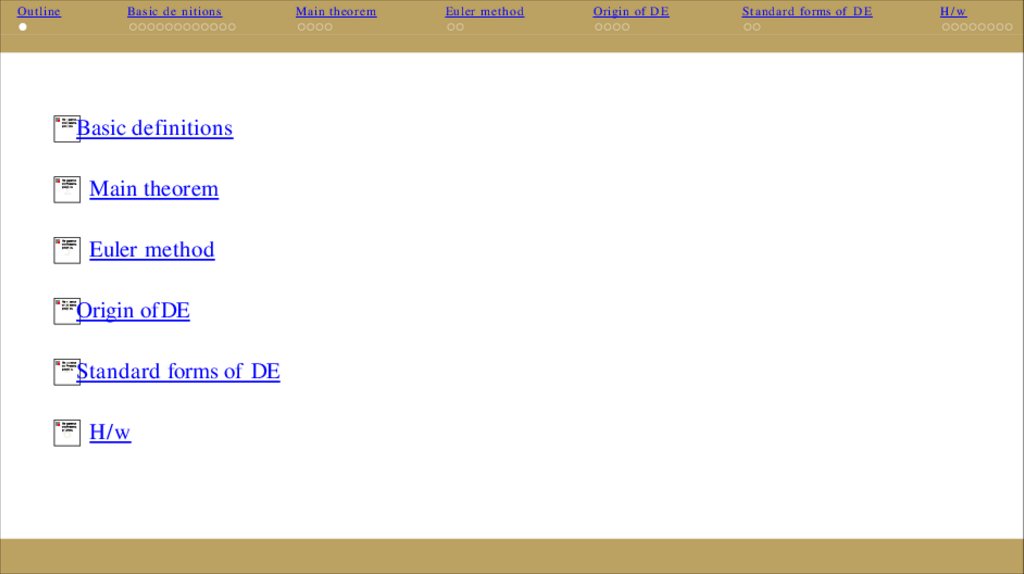
Outline
Basic de nitions
1
Basic definitions
2
Main theorem
3
Euler method
4
Origin ofDE
5
Standard forms of DE
6
H/w
Main theor em
Euler met hod
Origin of D E
Standar d forms of D E
H/w

3.

Outline
Basic de nitions
Main theor em
Euler met hod
Origin of D E
Standar d forms of D E
H/w
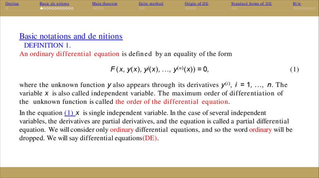
Basic notations and de nitions
DEFINITION 1.
An ordinary differential equation is defin e d by an equality of the form
F (x, y(x), y j (x), ..., y (n) (x)) = 0,
(1)
where the unknown function y also appears through its derivatives y (i) , i = 1, ..., n. The
variable x is also called independent variable. The maximum order of differentiation of
the unknown function is called the order of the differential equation.
In the equation (1) x is single independent variable. In the case of several independent
variables, the derivatives are partial derivatives, and the equation is called a partial differential
equation. We will consider only ordinary differential equations, and so the word ordinary will be
dropped. We will say differential equations(DE).

4.

Outline
Basic de nitions
Main theor em
Euler met hod
Origin of D E
Standar d forms of D E
H/w
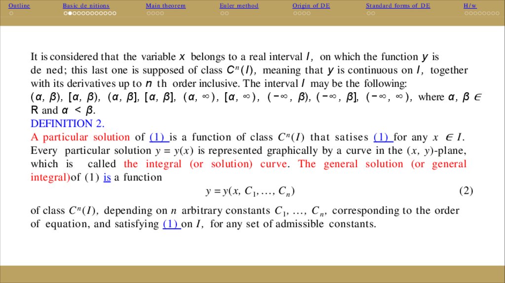
It is considered that the variable x belongs to a real interval I , on which the function y is
de ned; this last one is supposed of class C n (I), meaning that y is continuous on I , together
with its derivatives up to n t h order inclusive. The interval I may be the following:
(α, β), [α, β), (α, β], [α, β], (α, ∞ ) , [α, ∞ ) , ( − ∞ , β), ( − ∞ , β], ( − ∞ , ∞ ) , where α, β ∈
R and α < β.
DEFINITION 2.
A particular solution of (1) is a function of class C n ( I ) that satises (1) for any x ∈ I .
Every particular solution y = y(x) is represented graphically by a curve in the (x, y)-plane,
which is called the integral (or solution) curve. The general solution (or general
integral)of (1) is a function
y = y(x, C 1 , ..., C n )
(2)
of class C n ( I ) , depending on n arbitrary constants C 1 , ..., C n , corresponding to the order
of equation, and satisfying (1) on I , for any set of admissible constants.

5.

Outline
Basic de nitions
Main theor em
Euler met hod
Origin of D E
Standar d forms of D E
H/w
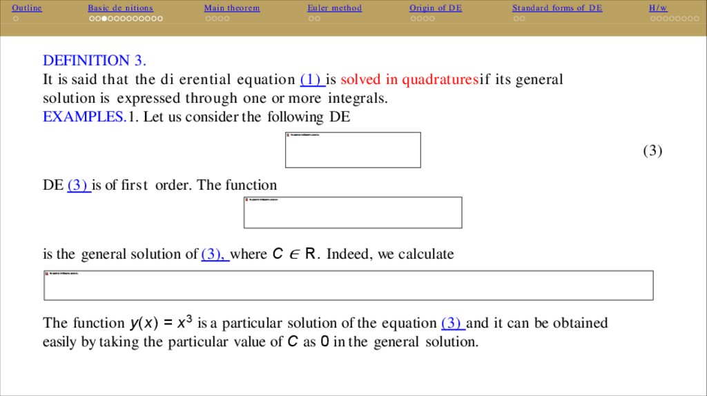
DEFINITION 3.
It is said that the di erential equation (1) is solved in quadraturesif its general
solution is expressed through one or more integrals.
EXAMPLES.1. Let us consider the following DE
(3)
DE (3) is of first order. The function
is the general solution of (3), where C ∈ R. Indeed, we calculate
The function y(x) = x 3 is a particular solution of the equation (3) and it can be obtained
easily by taking the particular value of C as 0 in the general solution.

6.

Outline
Basic de nitions
Main theor em
Euler met hod
Origin of D E
Standar d forms of D E
H/w
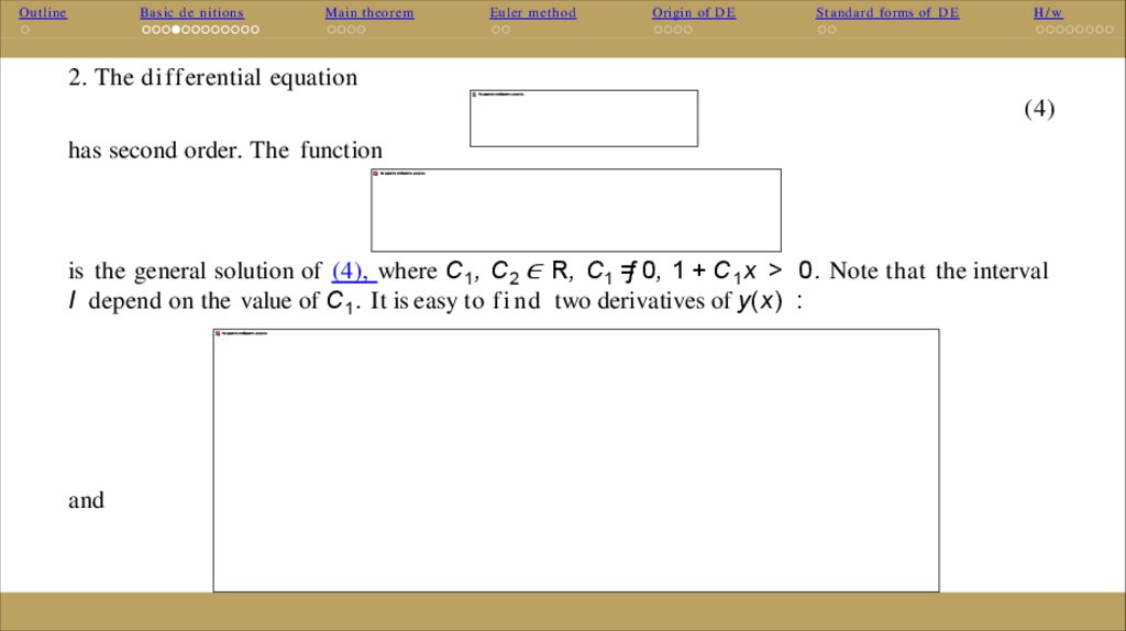
2. The differential equation
(4)
has second order. The function
is the general solution of (4), where C 1 , C2 ∈ R, C1 =ƒ 0, 1 + C 1 x > 0. Note that the interval
I depend on the value of C 1 . It is easy to f i n d two derivatives of y(x) :
and

7.

Outline
Basic de nitions
Main theor em
Euler met hod
Origin of D E
Standar d forms of D E
H/w
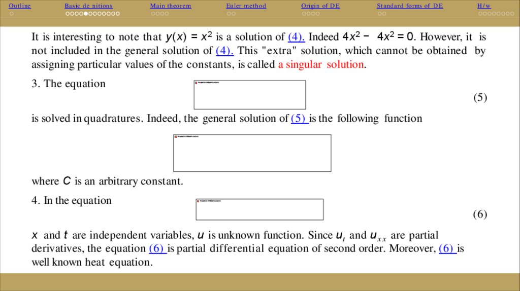
It is interesting to note that y(x) = x 2 is a solution of (4). Indeed 4x 2 − 4x 2 = 0. However, it is
not included in the general solution of (4). This "extra" solution, which cannot be obtained by
assigning particular values of the constants, is called a singular solution.
3. The equation
(5)
is solved in quadratures. Indeed, the general solution of (5) is the following function
where C is an arbitrary constant.
4. In the equation
(6)
x and t are independent variables, u is unknown function. Since u t and u x x are partial
derivatives, the equation (6) is partial differential equation of second order. Moreover, (6) is
well known heat equation.

8.

Outline
Basic de nitions
Main theor em
Euler met hod
Origin of D E
Standar d forms of D E
H/w
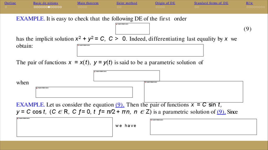
EXAMPLE. It is easy to check that the following DE of the first order
(9)
has the implicit solution x 2 + y 2 = C, C >
0. Indeed, differentiating last equality by x we
obtain:
The pair of functions x = x(t), y = y(t) is said to be a parametric solution of
when
EXAMPLE. Let us consider the equation (9). Then the pair of functions x = C sin t,
y = C cos t, (C ∈ R, C ƒ= 0, t ƒ= π/2 + πn, n ∈ Z) is a parametric solution of (9). Since
we have

9.

Outline
Basic de nitions
Main theor em
Euler met hod
Origin of D E
Standar d forms of D E
H/w
Some differential equations may be developed with respect to y (n) to give
(10)
We call this form normal. Most equations will be considered in normal form.
Di erential equations are classi ed into two groups: linear and nonlinear. A DE is said to be
linear if it is linear in y and all its derivatives. Thus, an n-th order linear DE has the form
(11)
DEFINITION 5.
In (11) if the function f (x) ≡ 0, then it is called a homogeneous DE, otherwise it is said to be
a nonhomogeneous DE. An equation that is not of the form (11) is a nonlinear DE.
Obviously, (3) is linear nonhomogeneous DE, whereas (4) is nonlinear homogeneous DE.

10.

Outline
Basic de nitions
Main theor em
Euler met hod
Origin of D E
Standar d forms of D E
H/w
In applications we are usually interested in a solution of the DE (10) satisfying some additional
requirements called initial or boundary conditions.
DEFINITION 6.
Byinitial conditions for (10) we mean n conditions of the form
(12)
where y 0 , ..., y n−1 and x 0 are given constants. A problem consisting of the DE (10) together
with the initial conditions (12) is called an initial value problem or the Cauchy problem.
It is common to seek a solution y(x) of the initial value problem (10), (12) in an interval I
which contains the point x 0 .

11.

Outline
Basic de nitions
Main theor em
Euler met hod
Origin of D E
Standar d forms of D E
DEFINITION 7.
If the conditions relate to two differen t x values, the problem is called a two-point
boundary-value problem(or simply a boundary-value problem).
We formulate two-point conditions for the n-th order DE (10):
where y(0) = y and α i j , β i j , γ i , i, j = 0, n − 1 are given constants and a, b ∈ I .
It is well known boundary-value problems is Sturm Liouville problems. Let us consider one of
them:
H/w

12.

Outline
Basic de nitions
Main theor em
Euler met hod
Origin of D E
Standar d forms of D E
H/w
EXAMPLES.
1) Consider the problem
Both of initial conditions relate to one x value, namely, x = 1. Thus this is an initial-value
problem. We will see later that this problem has a unique solution.
2) Consider the problem
In this problem we again seek a solution of the same di erential equation, but the conditions
relate to the two different x values, 0 and π/2. This is a (two-point) boundary-value problem.
This problem also has a unique solution; but the boundary-value problem
has no solution at all! This simple fact may lead one to the correct conclusion that
boundary-value problems are not to be taken lightly!

13.

Outline
Basic de nitions
Main theor em
Euler met hod
Origin of D E
Standar d forms of D E
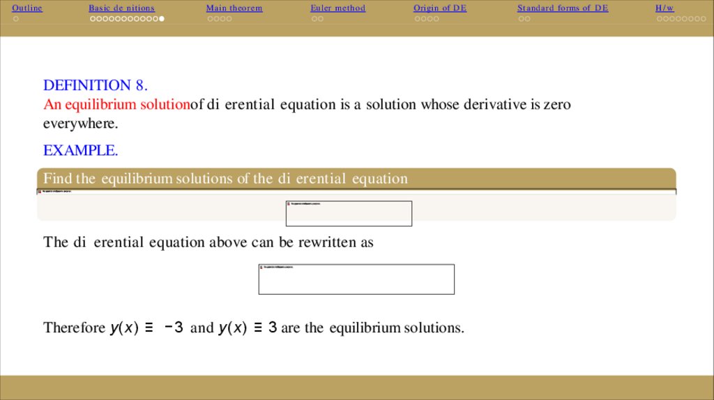
DEFINITION 8.
An equilibrium solutionof di erential equation is a solution whose derivative is zero
everywhere.
EXAMPLE.
Find the equilibrium solutions of the di erential equation
The di erential equation above can be rewritten as
Therefore y(x) ≡ −3 and y(x) ≡ 3 are the equilibrium solutions.
H/w

14.

Outline
Basic de nitions
Main theor em
Euler met hod
Origin of D E
Standar d forms of D E
H/w
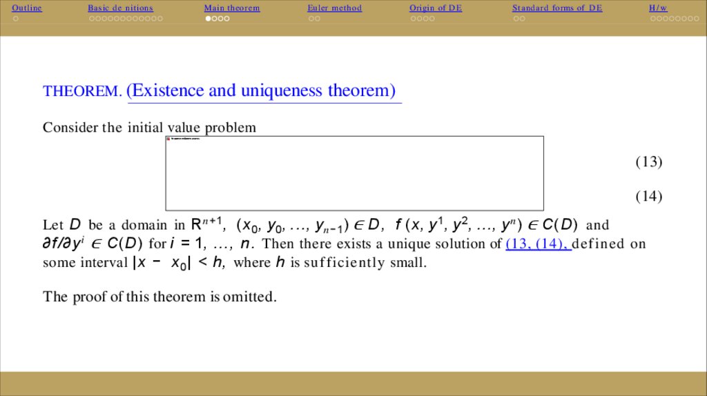
THEOREM. (Existence and uniqueness theorem)
Consider the initial value problem
(13)
(14)
Let D be a domain in R n+1 , (x 0 , y 0 , ..., y n−1 ) ∈ D , f (x, y 1 , y 2 , ..., y n ) ∈ C(D) and
∂f/∂y i ∈ C(D) for i = 1, ..., n. Then there exists a unique solution of (13, (14), defined on
some interval |x − x 0 | < h, where h is sufficiently small.
The proof of this theorem is omitted.

15.

Outline
Basic de nitions
Main theor em
Euler met hod
Origin of D E
Standar d forms of D E
H/w
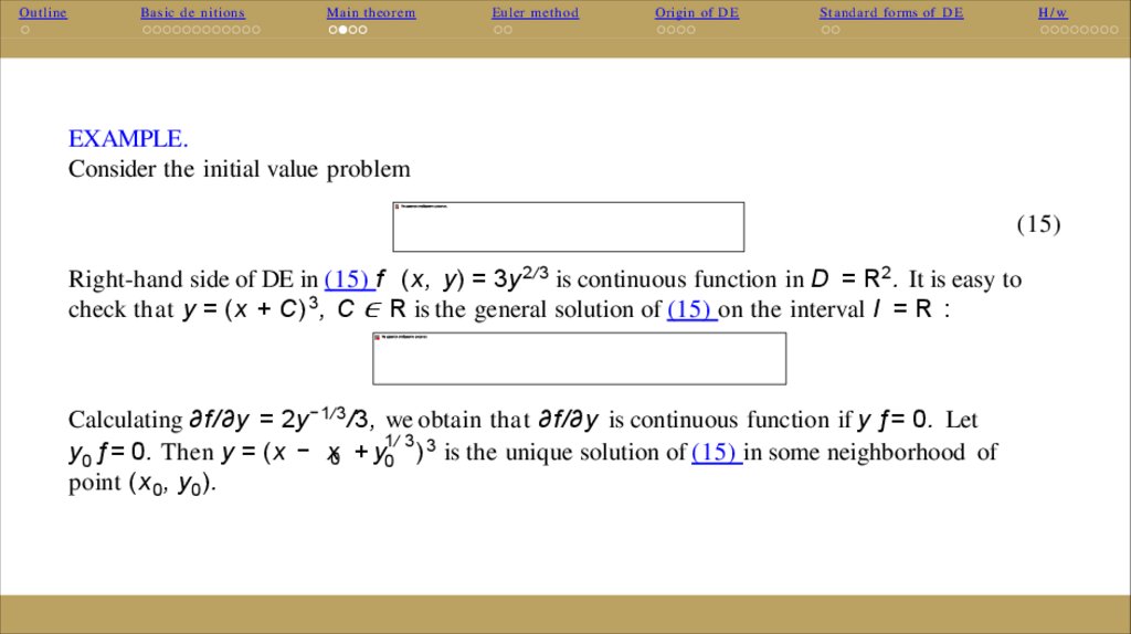
EXAMPLE.
Consider the initial value problem
(15)
Right-hand side of DE in (15) f (x, y) = 3y 2/3 is continuous function in D = R 2 . It is easy to
check that y = (x + C) 3 , C ∈ R is the general solution of (15) on the interval I = R :
Calculating ∂f/∂y = 2y −1/3 /3, we obtain that ∂f/∂y is continuous function if y ƒ= 0. Let
1/ 3
y0 ƒ= 0. Then y = (x − x0 + y0 ) 3 is the unique solution of (15) in some neighborhood of
point (x 0 , y0).

16.

Outline
Basic de nitions
Main theor em
Euler met hod
Origin of D E
Standar d forms of D E
On other hand, if y0 = 0 the problem (15) has the following solutions: y = (x − x 0 ) 3 and
y(x) ≡ 0. Moreover, the problem (15) has an in nite number of solutions:
where x any constant such that x > x 0 .
Let in (15) y(x 1 ) = y1 (as on the picture)
instead of y(x 0 ) = y 0 . What is a domain
of the uniqueness of this solution?
Answer: x ≤ x 0 .
H/w

17.

Outline
Basic de nitions
Main theor em
Euler met hod
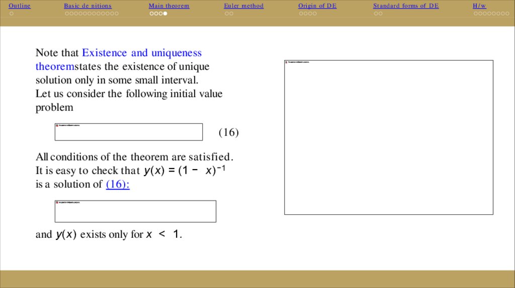
Note that Existence and uniqueness
theoremstates the existence of unique
solution only in some small interval.
Let us consider the following initial value
problem
(16)
All conditions of the theorem are satisfied.
It is easy to check that y(x) = (1 − x) −1
is a solution of (16):
and y(x) exists only for x < 1.
Origin of D E
Standar d forms of D E
H/w

18.

Outline
Basic de nitions
Main theor em
Euler met hod
Origin of D E
Standar d forms of D E
H/w
The Euler method
Although it is not always possible to n d an analytical solution of
(17)
for y = y(x), it is always possible to determine a numerical solution given an initial value y(x 0 ) =
y 0 , provided f (x, y) is a well-behaved function. The di erential equation (17) gives us the
slope f (x 0 , y0) of the tangent line to the solution curve y = y(x) at the point (x 0 , y 0).
With a small step size ∆x = x 1 − x 0 , the initial condition (x 0 , y0) can be marched forward to
(x 1 , y 1) along the tangent line using Euler's method (see Fig. 1)
y1 = y0 + ∆x f (x 0 , y 0).
Now (x 1 , y1) becomes the new initial condition and is marched forward to (x 2 , y 2) along a
newly determined tangent line with slope given by f (x 1 , y1) :
y2 = y1 + ∆x f (x 1 , y 1).
For small enough ∆x, the numerical solution converges to the exact solution.

19.

Outline
Basic de nitions
Main theor em
Euler met hod
Origin of D E
Standar d forms of D E
H/w

20.

Outline
Basic de nitions
Main theor em
Euler met hod
Origin of D E
Standar d forms of D E
Origin and applications of differential equations
The laws of the universe are written in the language of mathematics. Algebra is sufficient to
solve many static problems, but the most interesting natural phenomena involve change and
are described by equations that relate changing quantities.
Because the derivative
of the function f is the rate at which the quantity
y = f (t) is changing with respect to the independent variable t, it is natural that equations
involving derivatives are frequently used to describe the changing universe.
EXAMPLES.
1). As first example, consider a mass falling under the influence of constant gravity, such as
approximately found on the Earth's surface. Newton's law, F = ma, results in the equation
m
d2y
=−mg,
dt2
where y is the height of the object above the ground, m is the mass of the object, and
g ≈ 9.8meter/sec 2 is the constant gravitational acceleration.
H/w

21.

Outline
Basic de nitions
Main theor em
Euler met hod
Origin of D E
Standar d forms of D E
H/w
The mass cancels from the equation, and
d2y
dt2 =− g .
Here, the right-hand-side of the DE is a constant. The first integration yields
dy (t) = A − gt,
dt
with A the rst constant of integration. The second integration yields
gt 2
2
with B the second constant of integration. The two constants of integration A and B can then
be determined from the initial conditions. If we know that the initial height of the mass is y 0 , and
the initial velocity is v 0 , then the initial conditions are
y(t) = B + At −
y(0) = y 0 ,
dy
dt (0) = v 0 .

22.

Outline
Basic de nitions
Main theor em
Euler met hod
Origin of D E
Standar d forms of D E
H/w
Substitution of these initial conditions into the equations for dy/dt and y allows us to solve for
A and B :
dy (t) = A − gt =⇒ dy (0) = A = v ,
0
dt
dt
gt 2
=⇒ y(0) = B = y 0 .
2
The unique solution that satisfies both DE and the initial conditions is given by
y(t) = B + At −
gt 2
y(t) = y0 + v 0 t − 2 .
(18)
For example, suppose we drop a ball from the top of a 50 meter building. How long will it take
the ball to hit the ground? This question requires solution of (18) for the time T it takes for y(T )
= 0, given y0 = 50 meter and v 0 = 0. Solving for T,
.
.
100
gT 2
gT 2
y(T ) = y0 + v 0 T −
=⇒ 0 =50 −
=⇒ T =
≈
9.8 sec ≈
10
2
2
3.2sec.
0
g

23.

Outline
Basic de nitions
Main theor em
Euler met hod
Origin of D E
Standar d forms of D E
H/w
2). Newton's law of cooling may be stated in this way: The time rate of change (the rate of
change with respect to time t) of the temperature T (t) of a body is proportional to the
difference between T and the temperature A of the surrounding medium. That is,
dT = −k(T − A),
dt
where k is a positive constant. Observe that if T > A, then
, so the temperature is a
decreasing function of t and the body is cooling. But if T < A, then
, so that T is
increasing. Thus the physical law is translated into a di erential equation. If we are given the
values of k and A, initial temperature T (0) = T 0 , we are able to predict the future temperature
of the body by explicit formula:
T (t) = A + (T0 − A) exp(−kt).
Indeed,
dT = −k(T − A) exp(−kt) = − k [A + (T − A) exp(−kt) − A] = −k(T − A).
0
0
dt
Obviously, T (t) → A as t → ∞ .

24.

Outline
Basic de nitions
Main theor em
Euler met hod
Origin of D E
Standar d forms of D E
H/w
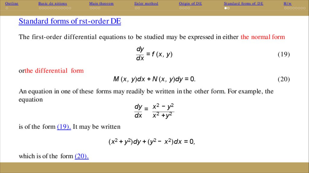
Standard forms of rst-order DE
The first-order differential equations to be studied may be expressed in either the normal form
dy
= f (x , y)
dx
(19)
M (x , y)dx + N (x , y)dy = 0.
(20)
orthe differential form
An equation in one of these forms may readily be written in the other form. For example, the
equation
dy = x 2 − y 2
dx
x 2 +y 2
is of the form (19). It may be written
(x 2 + y 2)dy + (y2 − x 2 )dx = 0,
which is of the form (20).

25.

Outline
Basic de nitions
Main theor em
Euler met hod
Origin of D E
Standar d forms of D E
H/w
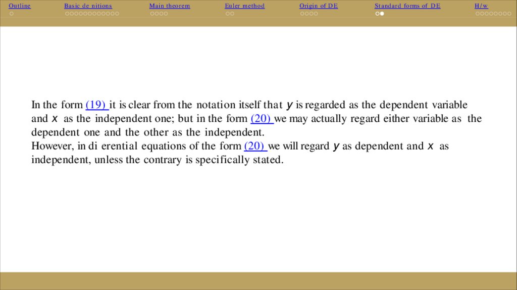
In the form (19) it is clear from the notation itself that y is regarded as the dependent variable
and x as the independent one; but in the form (20) we may actually regard either variable as the
dependent one and the other as the independent.
However, in di erential equations of the form (20) we will regard y as dependent and x as
independent, unless the contrary is specifically stated.

26.

Outline
Basic de nitions
Main theor em
Euler met hod
Origin of D E
Standar d forms of D E
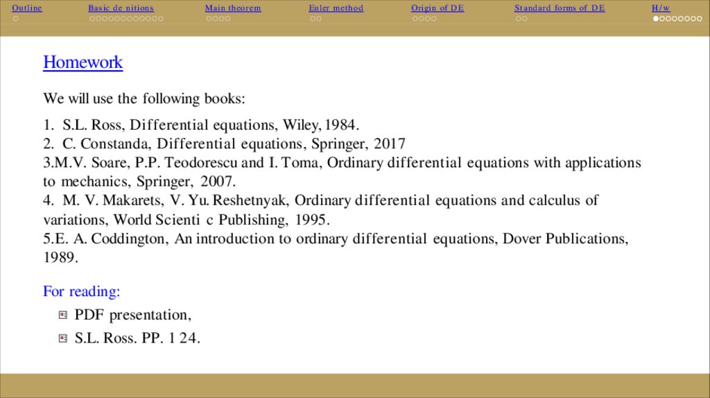
Homework
We will use the following books:
1. S.L. Ross, Differential equations, Wiley, 1984.
2. C. Constanda, Differential equations, Springer, 2017
3.M.V. Soare, P.P. Teodorescu and I. Toma, Ordinary differential equations with applications
to mechanics, Springer, 2007.
4. M. V. Makarets, V. Yu. Reshetnyak, Ordinary differential equations and calculus of
variations, World Scienti c Publishing, 1995.
5.E. A. Coddington, An introduction to ordinary differential equations, Dover Publications,
1989.
For reading:
PDF presentation,
S.L. Ross. PP. 1 24.
H/w

27.

Outline
Basic de nitions
Main theor em
Euler met hod
Origin of D E
Standar d forms of D E
Problems
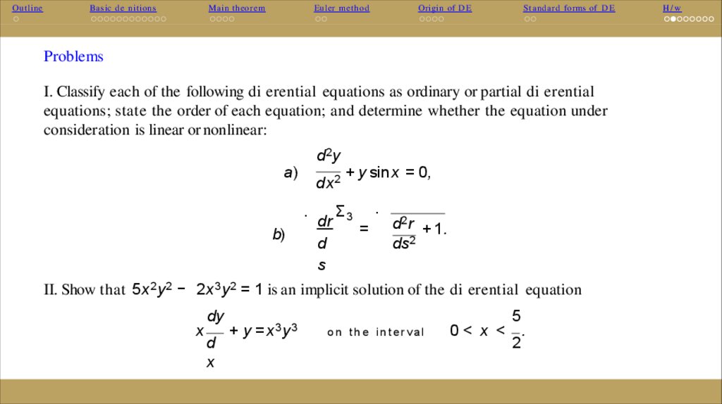
I. Classify each of the following di erential equations as ordinary or partial di erential
equations; state the order of each equation; and determine whether the equation under
consideration is linear or nonlinear:
d2y
a)
dx 2
.
b)
dr
d
s
+ y sinx = 0,
.
Σ3
=
d2 r + 1.
ds2
II. Show that 5x 2 y 2 − 2x 3 y 2 = 1 is an implicit solution of the di erential equation
x
dy
d
x
+ y =x 3 y 3
o n t h e in t e r val
0< x <
5
2
.
H/w

28.

Outline
Basic de nitions
Main theor em
Euler met hod
Origin of D E
Standar d forms of D E
H/w
III. Show that every function f de ned by f (x) = (x 3 + c) exp(−3x), where c is an arbitrary
constant, is a solution of the di erential equation
dy
+ 3y = 3x 2exp(−3x).
d
x
IV. For certain values of the constant m the function f de ned by f (x) = exp(mx) is a
solution of the di erential equation
d3y
d2y
dy
−
3
3
dx
dx 2 − 4 dx + 12y = 0.
Determine all such values of m .
V. Show that the function f de ned by f (x) = 3exp(2x) − 2x exp(2x) − cos(2x) satis es the
di erential equation
d2y
dy
dx 2 − 4 dx + 4y = −8 sin(2x).
and also the conditions that f (0) = 2 and f j (0) = 4.

29.

Outline
Basic de nitions
Main theor em
Euler met hod
Origin of D E
Standar d forms of D E
H/w
Extra materials
Direction elds
Very often, a nonlinear rst-order DE cannot be solved by means of integrals; therefore, to
obtain information about the behavior of its solutions we must resort to qualitative analysis
methods. One such technique is the sketching of so-called direction elds, based on the fact
that the right-hand side of the equation y j = f (x, y) is the slope of the tangent to the solution
curve y = y(x) at a point (x, y). Drawing short segments of the line with slope f (x, y) at each
node of a suitably chosen lattice in the (x, y)-plane, and examining the pattern formed by these
segments, we can build up a useful pictorial image of the family of solution curves of the given
DE.

30.

Outline
Basic de nitions
Main theor em
Euler met hod
Origin of D E
Standar d forms of D E
H/w

31.

Outline
Basic de nitions
Main theor em
Euler met hod
Origin of D E
Standar d forms of D E
H/w

32.

Outline
Basic de nitions
Main theor em
Euler met hod
Origin of D E
EXAMPLES OF DIRECTION FIELDS
Standar d forms of D E
H/w

33.

Outline
Basic de nitions
Main theor em
Euler met hod
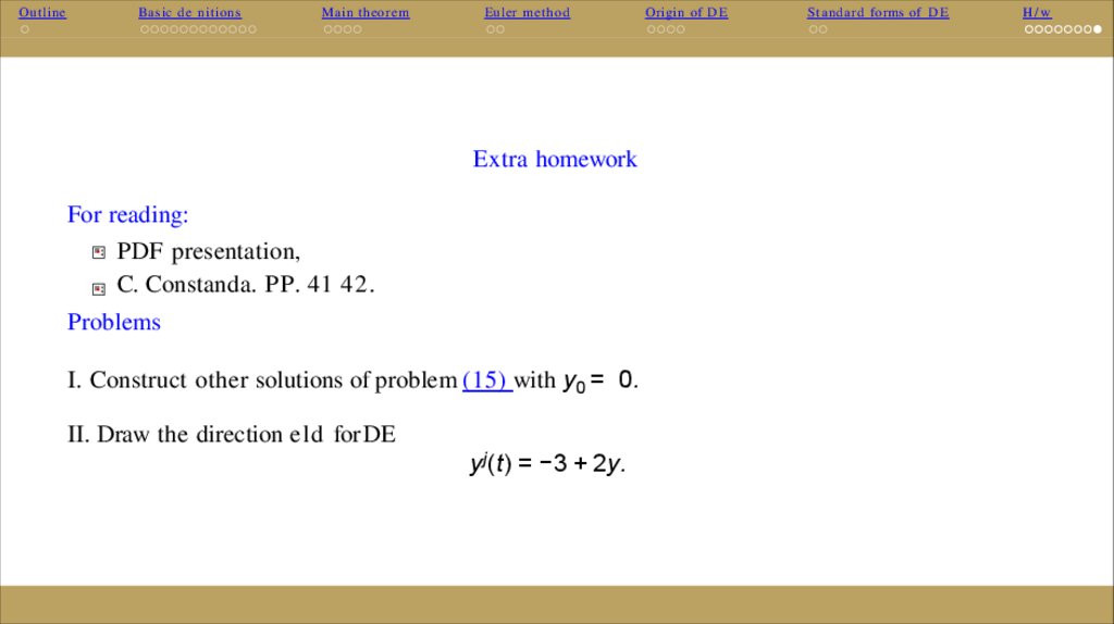
Extra homework
For reading:
PDF presentation,
C. Constanda. PP. 41 42.
Problems
I. Construct other solutions of problem (15) with y0 = 0.
II. Draw the direction eld for DE
y j (t) = −3 + 2y.
Origin of D E
Standar d forms of D E
H/w