


 Математика
Похожие презентации:


")


")


Multimachine Simulation. Lecture 20
1.
ECE 576 – Power SystemDynamics and Stability
Lecture 20: Multimachine Simulation
Prof. Tom Overbye
Dept. of Electrical and Computer Engineering
University of Illinois at Urbana-Champaign
overbye@illinois.edu
1
2.
Announcements• Read Chapter 7
• Homework 6 is due on Tuesday April 15
2
3.
Simultaneous Implicit• The other major solution approach is the simultaneous
implicit in which the algebraic and differential
equations are solved simultaneously
• This method has the advantage of being numerically
stable
3
4.
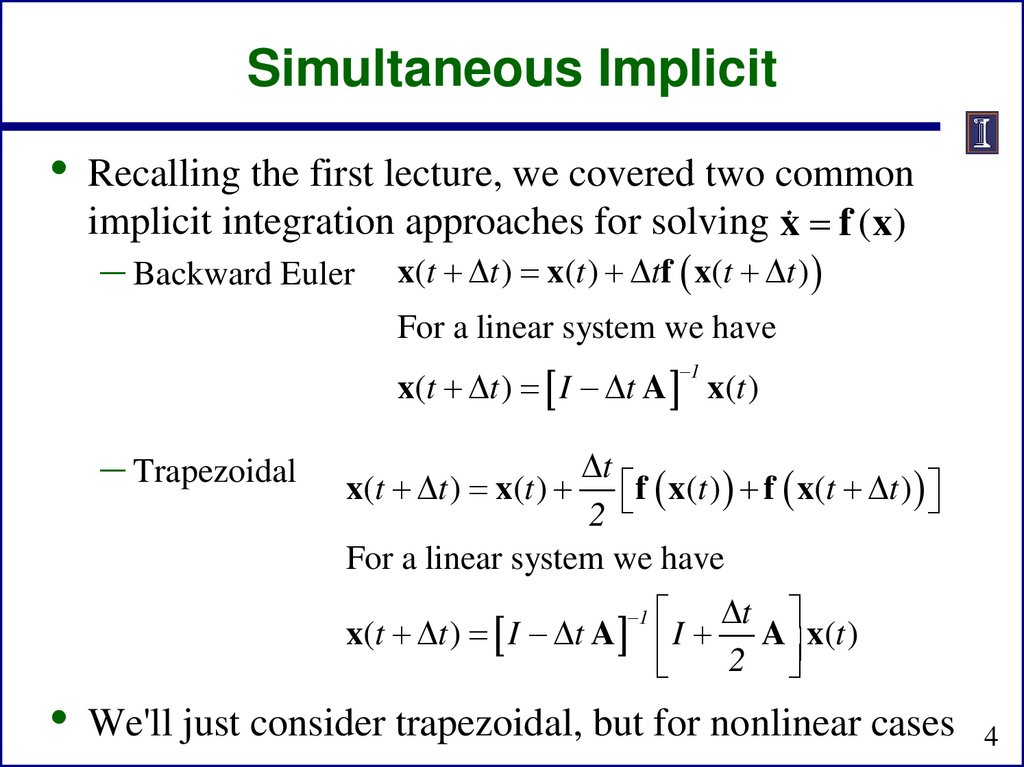
Simultaneous Implicit• Recalling the first lecture, we covered two common
implicit integration approaches for solving x f (x)
– Backward Euler
x(t t ) x(t ) tf x(t t )
For a linear system we have
x(t t ) I t A x(t )
1
– Trapezoidal
t
x(t t ) x(t ) f x(t ) f x(t t )
2
For a linear system we have
x(t t ) I t A
1
t
I 2 A x(t )
• We'll just consider trapezoidal, but for nonlinear cases 4
5.
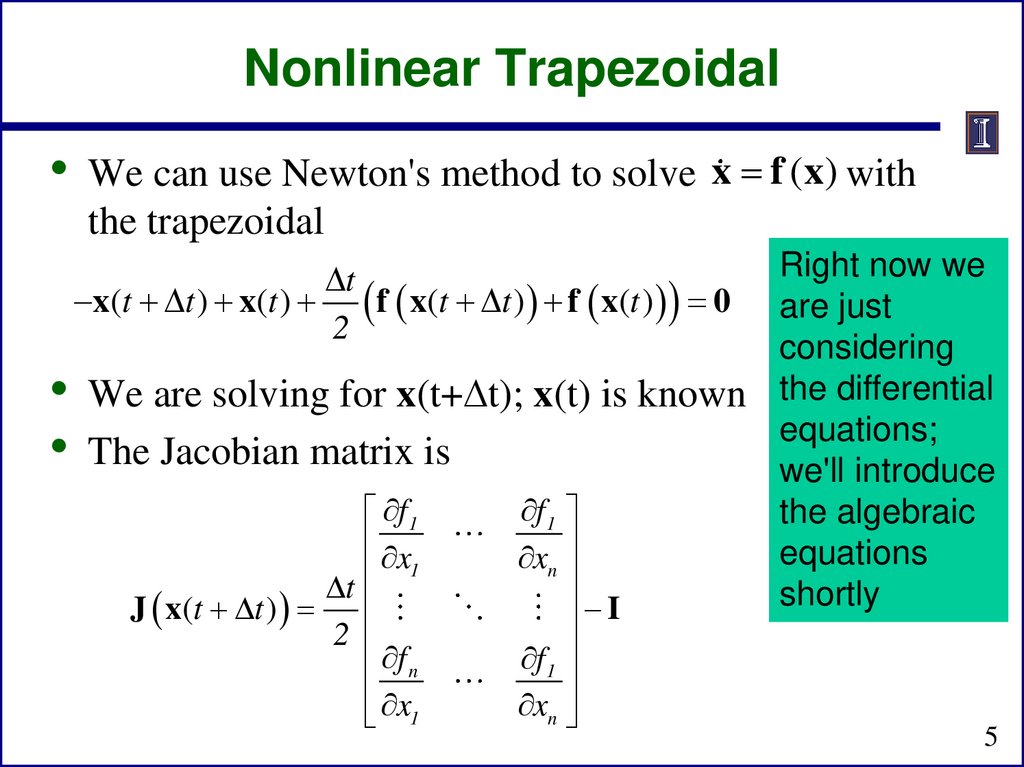
Nonlinear Trapezoidal• We can use Newton's method to solve x f (x) with
the trapezoidal
Right now we
are just
considering
We are solving for x(t+ t); x(t) is known the differential
equations;
The Jacobian matrix is
we'll introduce
f1
the algebraic
f1
x
equations
x
1
n
t
shortly
J x(t t )
I
2
f
f
1
n
x1
xn
t
x(t t ) x(t ) f x(t t ) f x(t ) 0
2
5
6.
Nonlinear Trapezoidal usingNewton's Method
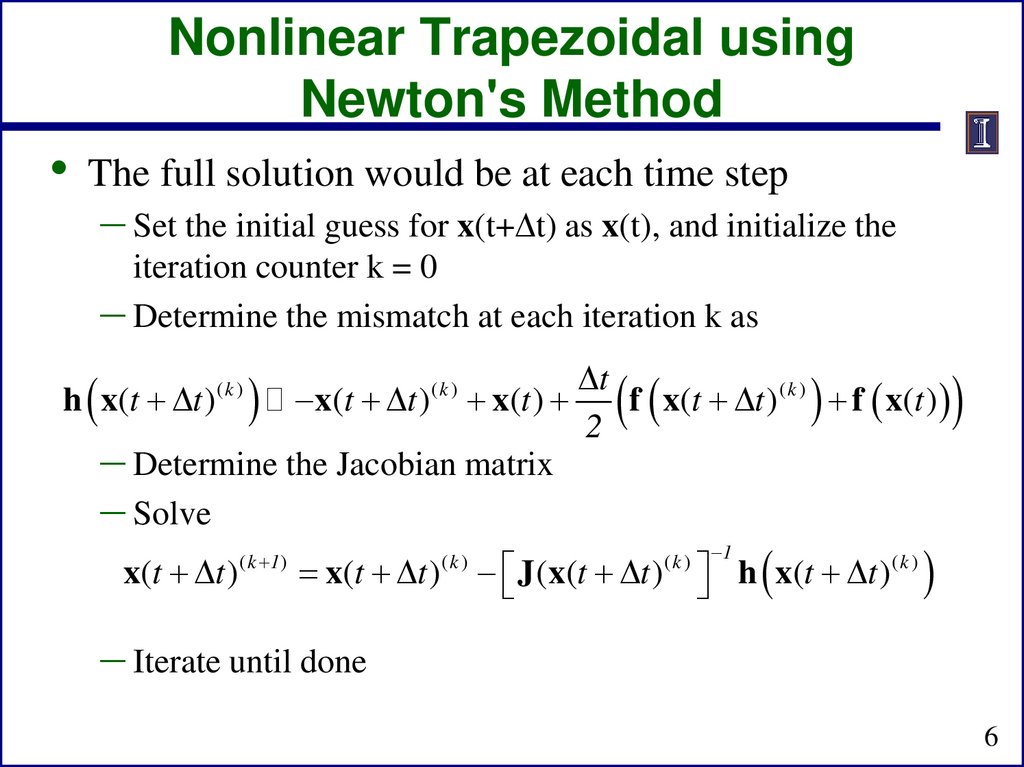
• The full solution would be at each time step
– Set the initial guess for x(t+ t) as x(t), and initialize the
iteration counter k = 0
– Determine the mismatch at each iteration k as
t
h x(t t ) x(t t ) x(t )
f x(t t ) ( k ) f x(t )
2
– Determine the Jacobian matrix
– Solve
(k )
x(t t )
( k 1)
(k )
x(t t )
(k )
J (x(t t ) h x(t t )( k )
(k )
1
– Iterate until done
6
7.
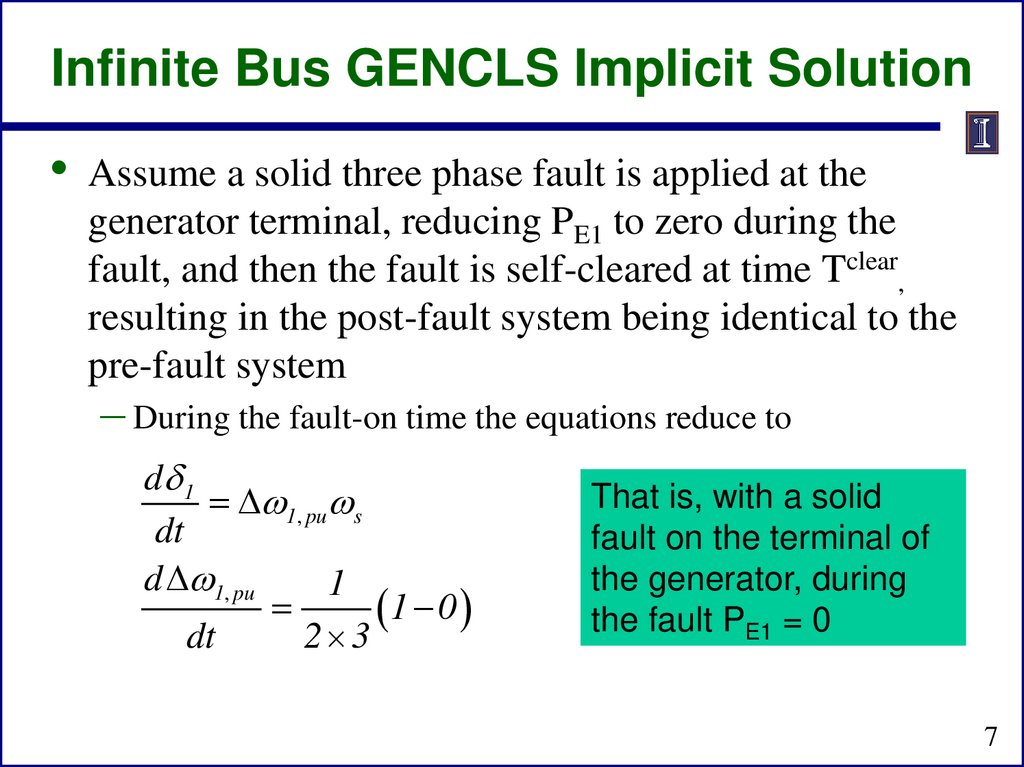
Infinite Bus GENCLS Implicit Solution• Assume a solid three phase fault is applied at the
generator terminal, reducing PE1 to zero during the
fault, and then the fault is self-cleared at time Tclear,
resulting in the post-fault system being identical to the
pre-fault system
– During the fault-on time the equations reduce to
d 1
1, pu s
dt
d 1, pu
1
1 0
dt
2 3
That is, with a solid
fault on the terminal of
the generator, during
the fault PE1 = 0
7
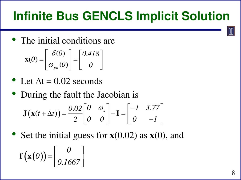
8.
Infinite Bus GENCLS Implicit Solution• The initial conditions are
(0 ) 0.418
x(0 )
(
0
)
0
pu
• Let t = 0.02 seconds
• During the fault the Jacobian is
1 3.77
0.02 0 s
J x(t t )
I
0
1
2 0 0
• Set the initial guess for x(0.02) as x(0), and
0
f x 0
0
.
1667
8
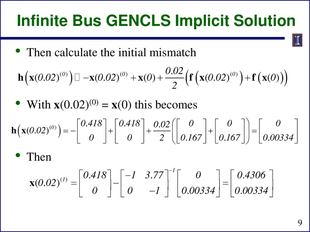
9.
Infinite Bus GENCLS Implicit Solution• Then calculate the initial mismatch
h x(0.02)(0 )
x(0.02) (0 ) x(0)
0.02
f x(0.02) (0 ) f x(0)
2
• With x(0.02)(0) = x(0) this becomes
0.418 0.418 0.02 0 0 0
h x(0.02)
2 0.167 0.167 0.00334
0 0
(0 )
• Then
1
x(0.02)
( 1)
0.418 1 3.77 0 0.4306
0
0
1
0
.
00334
0
.
00334
9
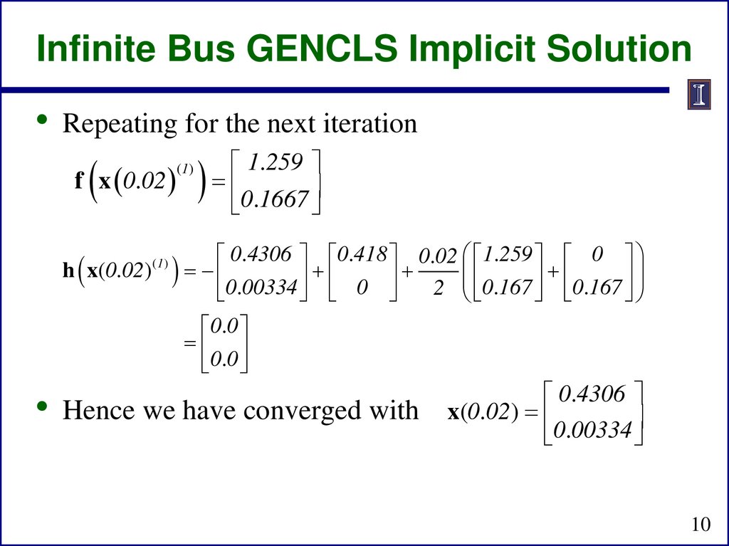
10.
Infinite Bus GENCLS Implicit Solution• Repeating for the next iteration
f x 0.02
( 1)
1.259
0
.
1667
0.4306 0.418 0.02 1.259 0
h x(0.02)
0
.
00334
0
0
.
167
0
.
167
2
( 1)
0.0
0.0
• Hence we have converged with
0.4306
x(0.02)
0
.
00334
10
11.
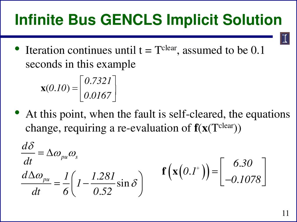
Infinite Bus GENCLS Implicit Solution• Iteration continues until t = Tclear, assumed to be 0.1
seconds in this example
0.7321
x(0.10 )
0
.
0167
• At this point, when the fault is self-cleared, the equations
change, requiring a re-evaluation of f(x(Tclear))
d
pu s
dt
d pu 1 1.281
1
sin
dt
6
0.52
6.30
f x 0 .1
0
.
1078
11
12.
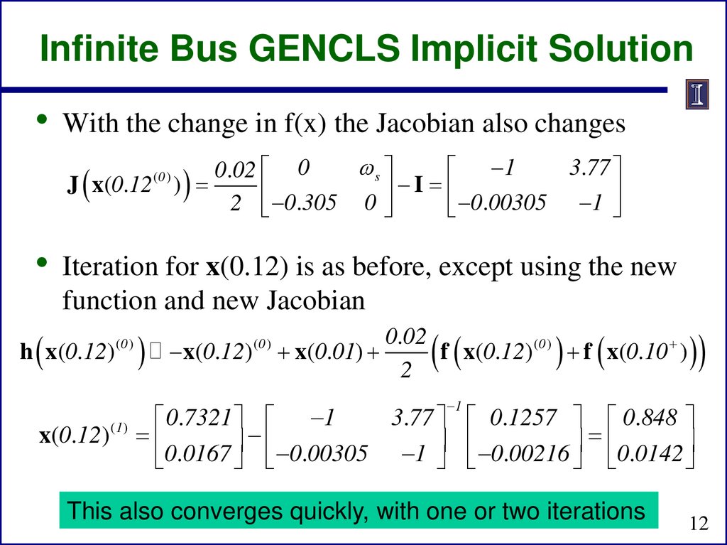
Infinite Bus GENCLS Implicit Solution• With the change in f(x) the Jacobian also changes
s
3.77
1
0.02 0
J x(0.12 )
I
0
.
00305
1
2 0.305 0
(0 )
• Iteration for x(0.12) is as before, except using the new
function and new Jacobian
h x(0.12)(0 )
x(0.12) (0 ) x(0.01)
0.02
f x(0.12) (0 ) f x(0.10 )
2
1
x(0.12)
( 1)
3.77 0.1257 0.848
0.7321 1
0
.
0167
0
.
00305
1
0
.
00216
0
.
0142
This also converges quickly, with one or two iterations
12
13.
Computational Considerations• As presented for a large system most of the
computation is associated with updating and factoring
the Jacobian. But the Jacobian actually changes little
and hence seldom needs to be rebuilt/factored
• Rather than using x(t) as the initial guess for x(t+ t),
prediction can be used when previous values are
available
x(t t )(0 ) x(t ) x(t ) x(t t )
13
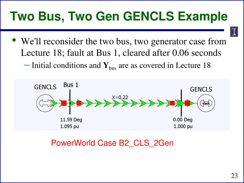
14.
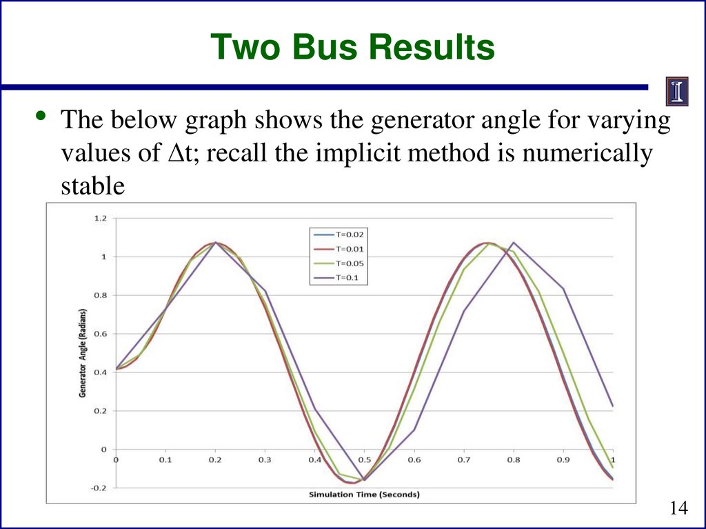
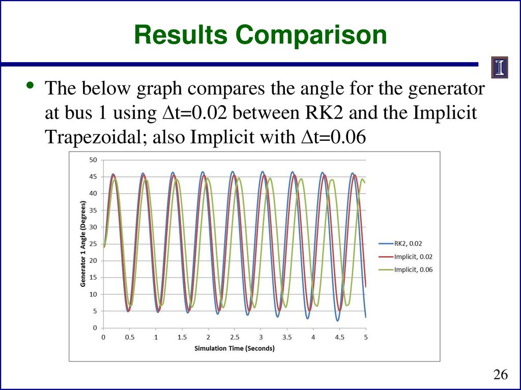
Two Bus Results• The below graph shows the generator angle for varying
values of t; recall the implicit method is numerically
stable
14
15.
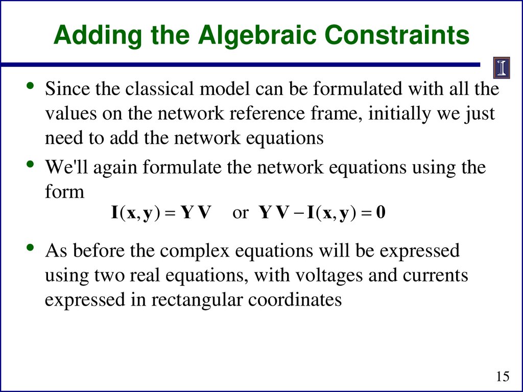
Adding the Algebraic Constraints• Since the classical model can be formulated with all the
values on the network reference frame, initially we just
need to add the network equations
• We'll again formulate the network equations using the
form
Ι (x, y ) Y V or Y V Ι (x, y ) 0
• As before the complex equations will be expressed
using two real equations, with voltages and currents
expressed in rectangular coordinates
15
16.
Adding the Algebraic Constraints• The network equations are as before
VD1
V
Q1
VD 2
y
VDn
VQn
n
G
V
B
V
I
(
x,y
)
0
1k QK
ND1
1k Dk
k 1
n
GikVQk BikVDK I NQ1 (x,y ) 0
k 1
n
G2 kVDk B2 kVQK I ND 2 (x,y ) 0
g (x, y ) k 1
n
G
V
B
V
I
(
x,y
)
0
nk QK
NDn
nk Dk
k 1
n
G
V
B
V
I
(
x,y
)
0
nk DK
NQn
nk Qk
k 1
16
17.
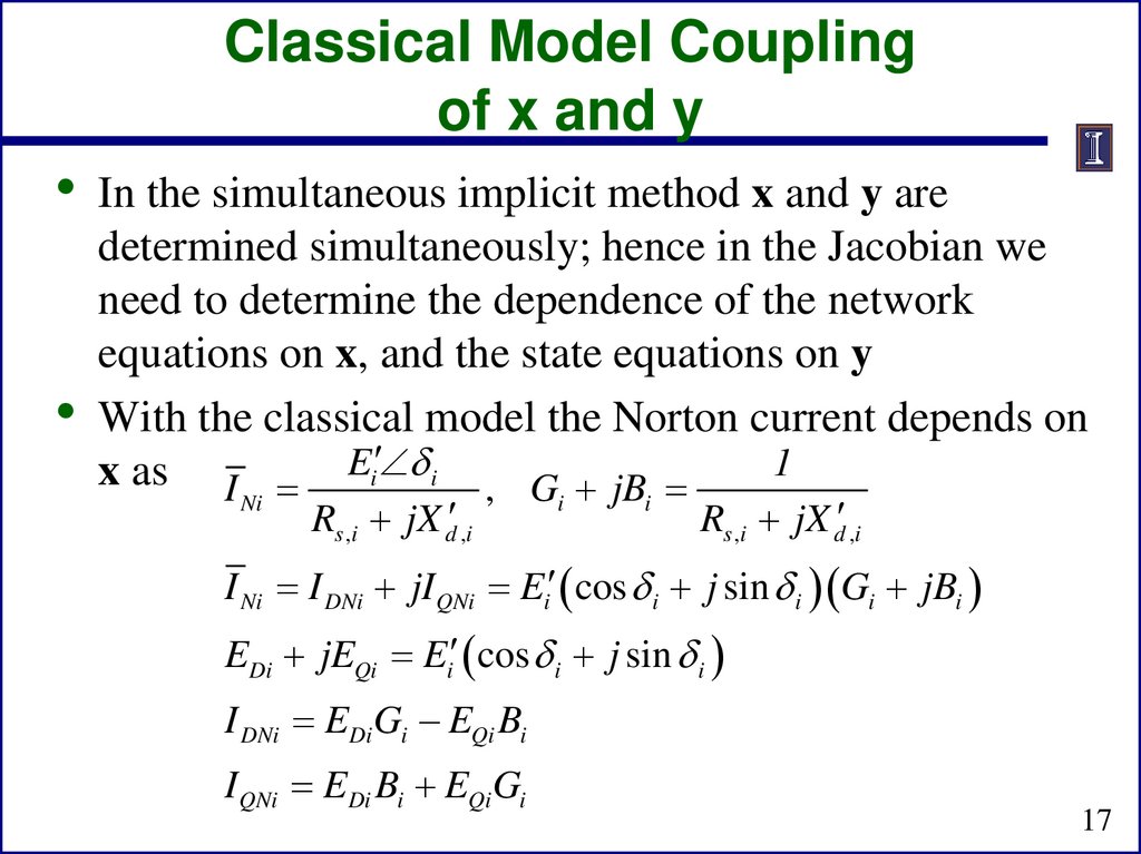
Classical Model Couplingof x and y
• In the simultaneous implicit method x and y are
determined simultaneously; hence in the Jacobian we
need to determine the dependence of the network
equations on x, and the state equations on y
• With the classical model the Norton current depends on
1
x as I Ei i , G jB
Ni
Rs ,i jX d ,i
i
i
Rs ,i jX d ,i
I Ni I DNi jI QNi Ei cos i j sin i Gi jBi
EDi jEQi Ei cos i j sin i
I DNi EDi Gi EQi Bi
I QNi EDi Bi EQi Gi
17
18.
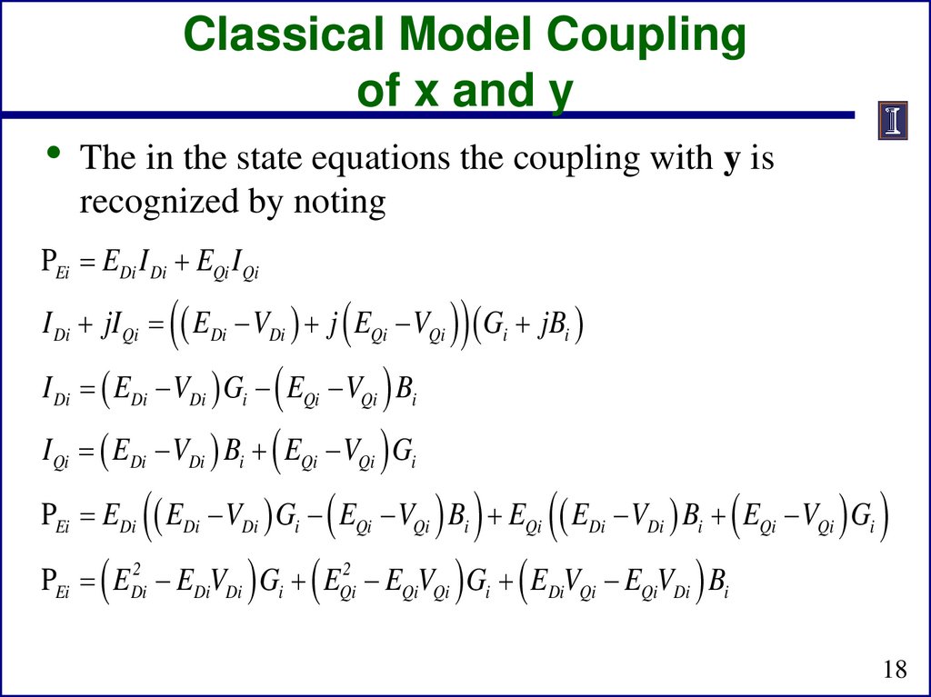
Classical Model Couplingof x and y
• The in the state equations the coupling with y is
recognized by noting
PEi EDi I Di EQi I Qi
I Di jI Qi EDi VDi j EQi VQi Gi jBi
I Di EDi VDi Gi EQi VQi Bi
I Qi EDi VDi Bi EQi VQi Gi
PEi EDi EDi VDi Gi EQi VQi Bi EQi EDi VDi Bi EQi VQi Gi
PEi EDi2 EDiVDi Gi EQi2 EQiVQi Gi EDiVQi EQiVDi Bi
18
19.
Variables and Mismatch Equations• In solving the Newton algorithm the variables now
include x and y (recalling that here y is just the vector
of the real and imaginary bus voltages
• The mismatch equations now include the state
integration equations
h x(t t )( k )
x(t t )
(k )
t
x(t )
f x(t t ) ( k ) , y (t t ) ( k ) f x(t ), y (t )
2
• And the algebraic equations
g x(t t ) , y (t t )
(k )
(k )
19
20.
Jacobian Matrix• Since the h(x,y) and g(x,y) are coupled, the Jacobian is
J x(t t ) , y (t t )
h x(t t ) , y (t t ) h x(t t ) , y (t t )
(k )
(k )
(k )
(k )
x
(k )
(k )
g
x
(
t
t
)
,
y
(
t
t
)
x
(k )
(k )
y
(k )
(k )
g x(t t ) , y (t t )
y
– With the classical model the coupling is the Norton current at
bus i depends on i (i.e., x) and the electrical power (PEi) in
the swing equation depends on VDi and VQi (i.e., y)
20
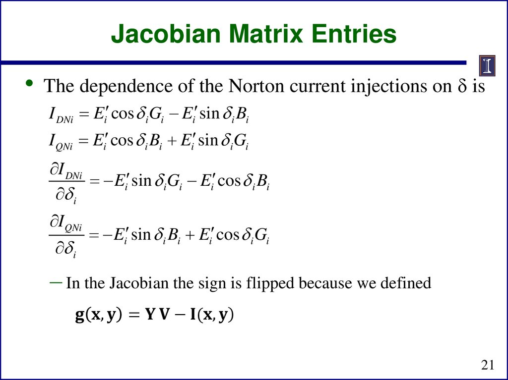
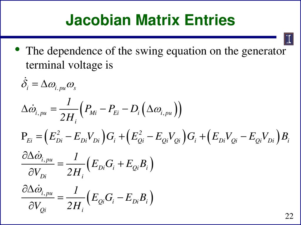
21.
Jacobian Matrix Entries• The dependence of the Norton current injections on is
I DNi Ei cos i Gi Ei sin i Bi
I QNi Ei cos i Bi Ei sin i Gi
I DNi
Ei sin i Gi Ei cos i Bi
i
I QNi
i
Ei sin i Bi Ei cos i Gi
– In the Jacobian the sign is flipped because we defined