


 Математика
Похожие презентации:

")

")


")


Discrete probability distributions (chapter 5)
1.
CHAPTER 5STATISTICS FOR BUSINESS AND ECONOMICS 13e Anderson,
David R 2017
2.
Discrete Probability DistributionsRANDOM VARIABLES
DEVELOPING DISCRETE
PROBABILITY
DISTRIBUTION
EXPECTED VALUE AND
VARIANCE
BIVARIATE AND
BINOMIAL
DISTRIBUTIONS
HYPERGEOMETRIC
PROBABILITY
DISTRIBUTION
3.
Statistics in Practice■ One of the largest banks in the world
■ Offers a wide range of financial services including
checking and saving accounts, loans and mortgages,
insurance, and investment services
■ One of the first banks in the United States to introduce
automatic teller machines (ATMs)
■ It lets customers do all of their banking in one place with
the touch of a finger, 24 hours a day, 7 days a week. More
than 150 different banking functions—from deposits to
managing investments—can be performed with ease.
■ Citibank customers use ATMs for 80% of their
transactions
4.
Statistics in Practice■ Challenge: Waiting Lines
■ Periodic capacity studies are used to analyze customer waiting times and to determine
whether additional ATMs are needed
■ Data collected showed that the random customer arrivals followed a probability distribution
known as the Poisson distribution
■ Using the Poisson distribution, Citibank can compute probabilities for the number of
customers arriving at a CBC during any time period and make decisions concerning the
number of ATMs needed
5.
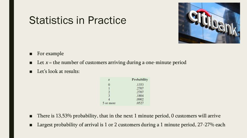
Statistics in Practice■ For example
■ Let x = the number of customers arriving during a one-minute period
■ Let’s look at results:
■ There is 13,53% probability, that in the next 1 minute period, 0 customers will arrive
■ Largest probability of arrival is 1 or 2 customers during a 1 minute period, 27-27% each
6.
Statistics in Practice■ Discrete probability distributions, such as the one used by Citibank, are the topic of this
chapter. In addition to the Poisson distribution, you will learn about the binomial and
hypergeometric distributions and how they can be used to provide helpful probability
information
7.
1. Random Variables■ A random variable is a numerical description of the outcome of an experiment.
■ In effect, a random variable associates a numerical value with each possible
experimental outcome
■ The particular numerical value of the random variable depends on the outcome of
the experiment
■ Depending on the numerical values it assumes, a random variable can be classified as
being either
– discrete
– or continuous
8.
1. Random VariablesDiscrete Random Variables
■ Random variable that may assume either a finite number of values or an infinite
sequence of values such as 0, 1, 2, . . .
■ For example, consider the experiment of an accountant taking the certified public
accountant (CPA) examination.
■ The examination has four parts. we can define a random variable as x = the number
of parts of the CPA examination passed
■ It is a discrete random variable because it may assume the finite number of values 0,
1, 2, 3, or 4.
9.
1. Random VariablesDiscrete Random Variables
■ Although the outcomes of many experiments can naturally be described by
numerical values, others cannot
■ For example, a survey question might ask an individual to recall the message in a
recent television commercial
■ Two possible outcomes: The individual cannot recall the message and the individual
can recall the message
■ We can still describe these experimental outcomes numerically by defining the
discrete random variable x as follows: let x = 0 if the individual cannot recall the
message and x = 1 if the individual can recall the message
10.
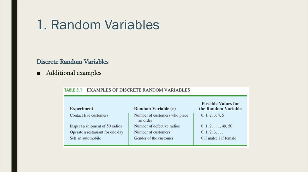
1. Random VariablesDiscrete Random Variables
■ Additional examples
11.
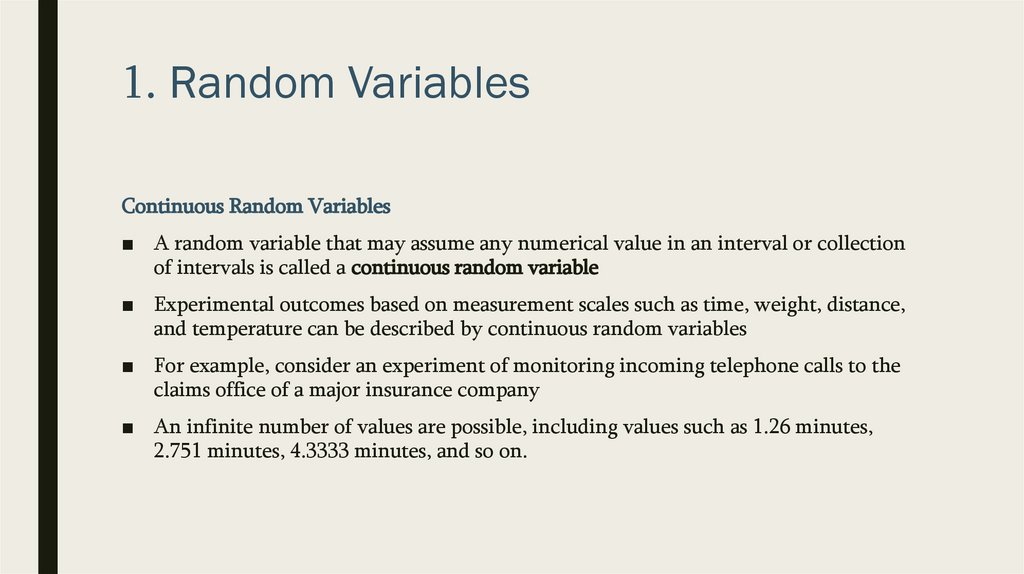
1. Random VariablesContinuous Random Variables
■ A random variable that may assume any numerical value in an interval or collection
of intervals is called a continuous random variable
■ Experimental outcomes based on measurement scales such as time, weight, distance,
and temperature can be described by continuous random variables
■ For example, consider an experiment of monitoring incoming telephone calls to the
claims office of a major insurance company
■ An infinite number of values are possible, including values such as 1.26 minutes,
2.751 minutes, 4.3333 minutes, and so on.
12.
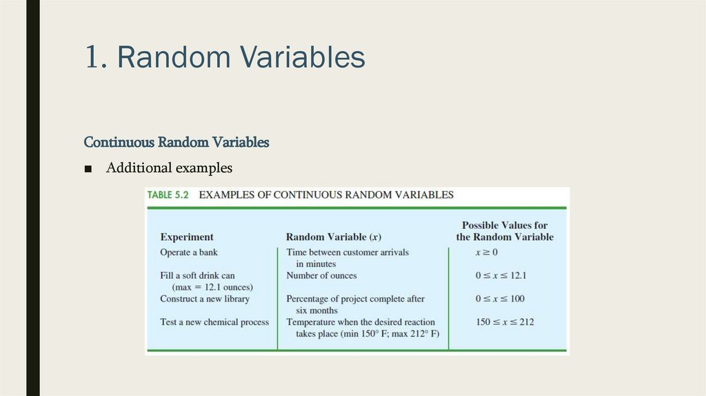
1. Random VariablesContinuous Random Variables
■ Additional examples
13.
2. Discrete Probability Distributions■ The probability distribution for a random variable describes how probabilities are
distributed over the values of the random variable
■ For a discrete random variable x, a probability function, denoted by f (x), provides
the probability for each value of the random variable
■ As such, you might suppose that the classical, subjective, and relative frequency
methods of assigning probabilities introduced in previous chapter would be useful in
developing discrete probability distributions
14.
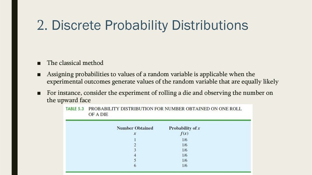
2. Discrete Probability Distributions■ The classical method
■ Assigning probabilities to values of a random variable is applicable when the
experimental outcomes generate values of the random variable that are equally likely
■ For instance, consider the experiment of rolling a die and observing the number on
the upward face
15.
2. Discrete Probability Distributions■ The subjective method
■ Assigning probabilities can also lead to a table of values of the random variable
together with the associated probabilities
■ With the subjective method the individual developing the probability distribution
uses their best judgment to assign each probability
16.
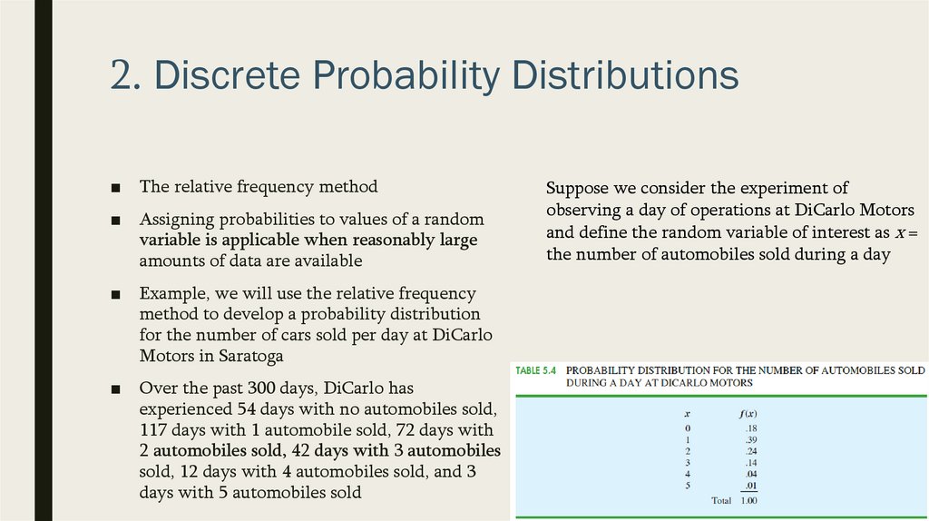
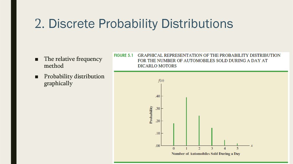
2. Discrete Probability Distributions■ The relative frequency method
■ Assigning probabilities to values of a random
variable is applicable when reasonably large
amounts of data are available
■ Example, we will use the relative frequency
method to develop a probability distribution
for the number of cars sold per day at DiCarlo
Motors in Saratoga
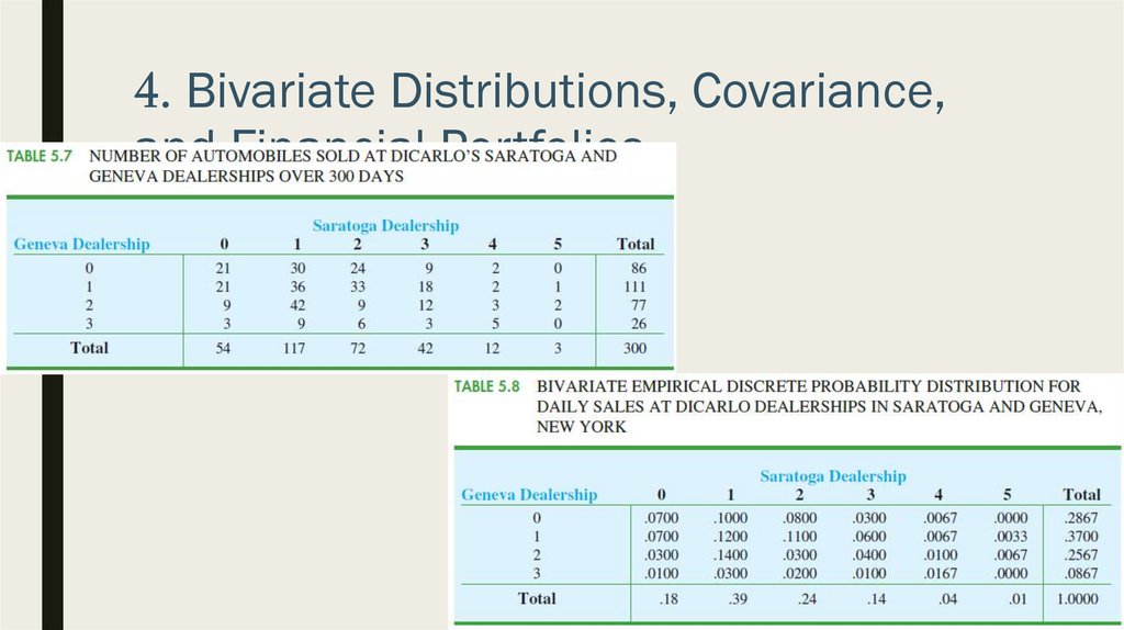
■ Over the past 300 days, DiCarlo has
experienced 54 days with no automobiles sold,
117 days with 1 automobile sold, 72 days with
2 automobiles sold, 42 days with 3 automobiles
sold, 12 days with 4 automobiles sold, and 3
days with 5 automobiles sold
Suppose we consider the experiment of
observing a day of operations at DiCarlo Motors
and define the random variable of interest as x =
the number of automobiles sold during a day
17.
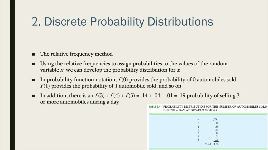
2. Discrete Probability Distributions■ The relative frequency method
■ Using the relative frequencies to assign probabilities to the values of the random
variable x, we can develop the probability distribution for x
■ In probability function notation, f (0) provides the probability of 0 automobiles sold,
f (1) provides the probability of 1 automobile sold, and so on
■ In addition, there is an f (3) + f (4) + f (5) = .14 + .04 + .01 = .19 probability of selling 3
or more automobiles during a day
18.
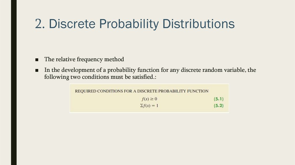
2. Discrete Probability Distributions■ The relative frequency method
■ In the development of a probability function for any discrete random variable, the
following two conditions must be satisfied.:
19.
2. Discrete Probability Distributions■ The relative frequency
method
■ Probability distribution
graphically
20.
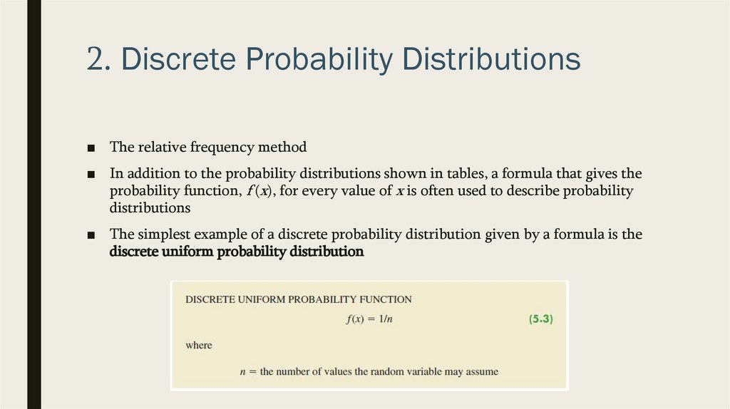
2. Discrete Probability Distributions■ The relative frequency method
■ In addition to the probability distributions shown in tables, a formula that gives the
probability function, f (x), for every value of x is often used to describe probability
distributions
■ The simplest example of a discrete probability distribution given by a formula is the
discrete uniform probability distribution
21.
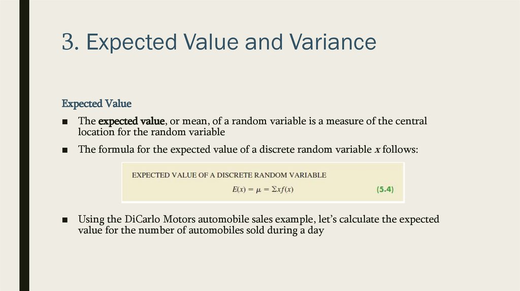
3. Expected Value and VarianceExpected Value
■ The expected value, or mean, of a random variable is a measure of the central
location for the random variable
■ The formula for the expected value of a discrete random variable x follows:
■ Using the DiCarlo Motors automobile sales example, let’s calculate the expected
value for the number of automobiles sold during a day
22.
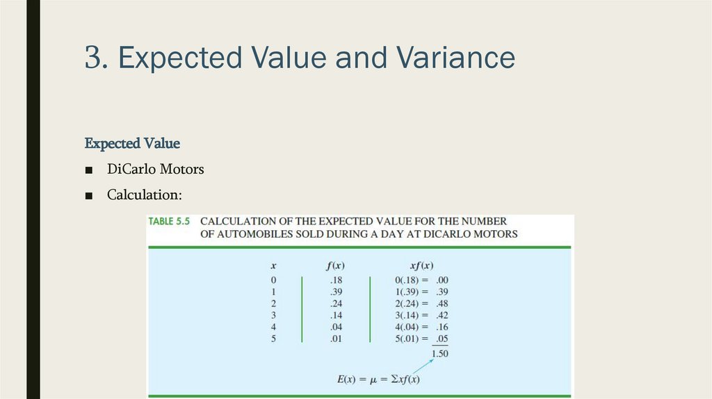
3. Expected Value and VarianceExpected Value
■ DiCarlo Motors
■ Calculation:
23.
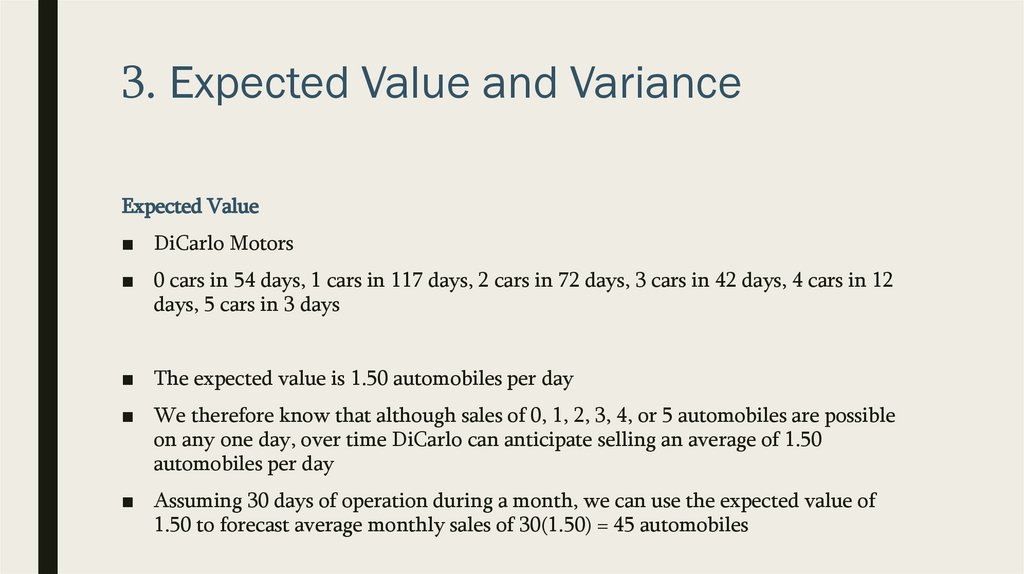
3. Expected Value and VarianceExpected Value
■ DiCarlo Motors
■ 0 cars in 54 days, 1 cars in 117 days, 2 cars in 72 days, 3 cars in 42 days, 4 cars in 12
days, 5 cars in 3 days
■ The expected value is 1.50 automobiles per day
■ We therefore know that although sales of 0, 1, 2, 3, 4, or 5 automobiles are possible
on any one day, over time DiCarlo can anticipate selling an average of 1.50
automobiles per day
■ Assuming 30 days of operation during a month, we can use the expected value of
1.50 to forecast average monthly sales of 30(1.50) = 45 automobiles
24.
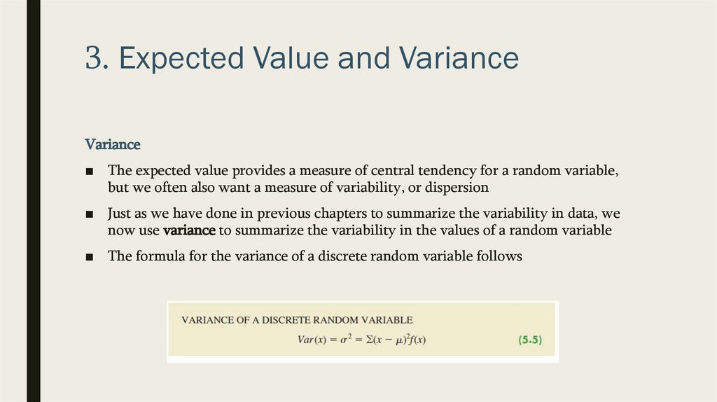
3. Expected Value and VarianceVariance
■ The expected value provides a measure of central tendency for a random variable,
but we often also want a measure of variability, or dispersion
■ Just as we have done in previous chapters to summarize the variability in data, we
now use variance to summarize the variability in the values of a random variable
■ The formula for the variance of a discrete random variable follows
25.
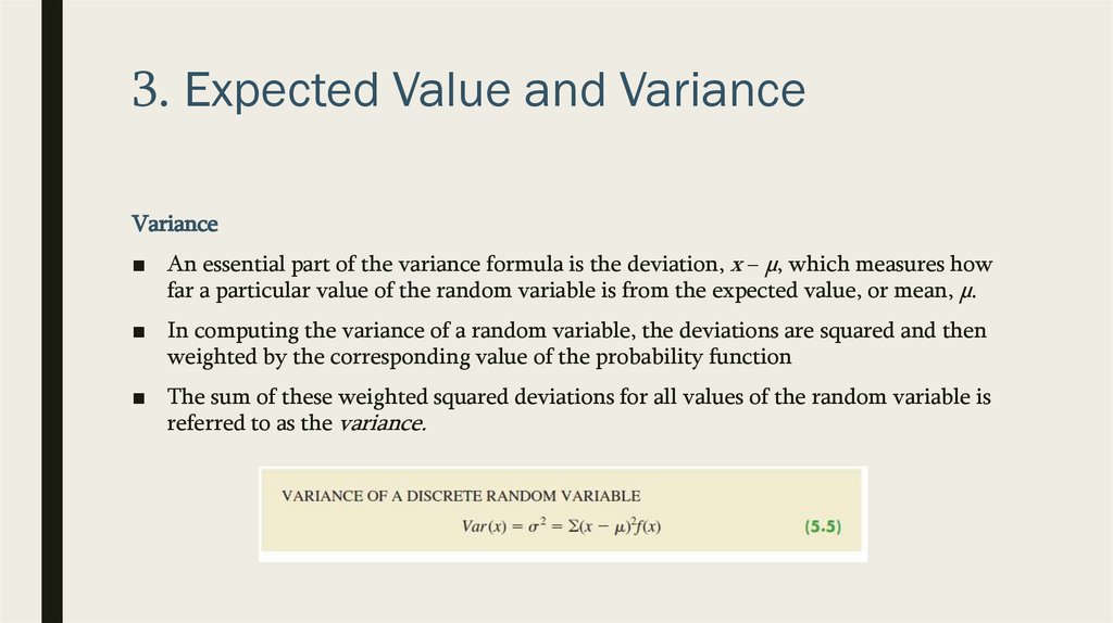
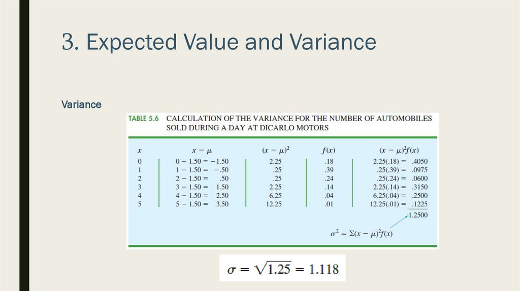
3. Expected Value and VarianceVariance
■ An essential part of the variance formula is the deviation, x − µ, which measures how
far a particular value of the random variable is from the expected value, or mean, µ.
■ In computing the variance of a random variable, the deviations are squared and then
weighted by the corresponding value of the probability function
■ The sum of these weighted squared deviations for all values of the random variable is
referred to as the variance.
26.
3. Expected Value and VarianceVariance
■ The standard deviation, σ, is defined as the positive square root of the variance
■ DiCarlo Motors example
27.
3. Expected Value and VarianceVariance
28.
4. Bivariate Distributions, Covariance,and Financial Portfolios
■ A probability distribution involving two random variables is called a bivariate
probability distribution
■ Each outcome for a bivariate experiment consists of two values, one for each random
variable
■ For example,
– Rolling a pair of dice
– Observing the financial markets for a year and recording the percentage gain
for a stock fund and a bond fund
29.
4. Bivariate Distributions, Covariance,and Financial Portfolios
■ When dealing with bivariate probability distributions, we are often interested in the
relationship between the random variables
■ We introduce bivariate distributions and show how the covariance and correlation
coefficient can be used as a measure of linear association between the random
variables
30.
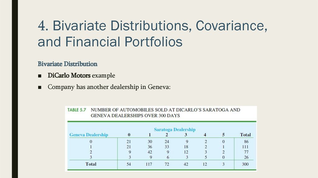
4. Bivariate Distributions, Covariance,and Financial Portfolios
Bivariate Distribution
■ DiCarlo Motors example
■ Company has another dealership in Geneva:
31.
4. Bivariate Distributions, Covariance,and Financial Portfolios
Bivariate Distribution
■ DiCarlo Motors example
■ Suppose we consider the bivariate experiment of observing a day of operations at
DiCarlo Motors and recording the number of cars sold
■ Let us define
– X = number of cars sold at the Geneva dealership and
– Y = number of cars sold at the Saratoga dealership
■ Let’s develop bivariate probabilities, often called joint probabilities
32.
4. Bivariate Distributions, Covariance,and Financial Portfolios
Bivariate Distribution
■ DiCarlo Motors example
33.
4. Bivariate Distributions, Covariance,and Financial Portfolios
Bivariate Distribution
■ „DiCarlo Motors example
■ The joint probability of selling 0 automobiles at Geneva and 1 automobile at Saratoga
on a typical day is f (0, 1) = .1000
34.
4. Bivariate Distributions, Covariance,and Financial Portfolios
Bivariate Distribution
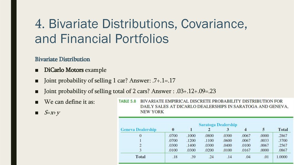
■ DiCarlo Motors example
■ Joint probability of selling 1 car? Answer: .7+.1=.17
■ Joint probability of selling total of 2 cars? Answer : .03+.12+.09=.23
■ We can define it as:
■ S=x+y
35.
4. Bivariate Distributions, Covariance,and Financial Portfolios
Bivariate Distribution
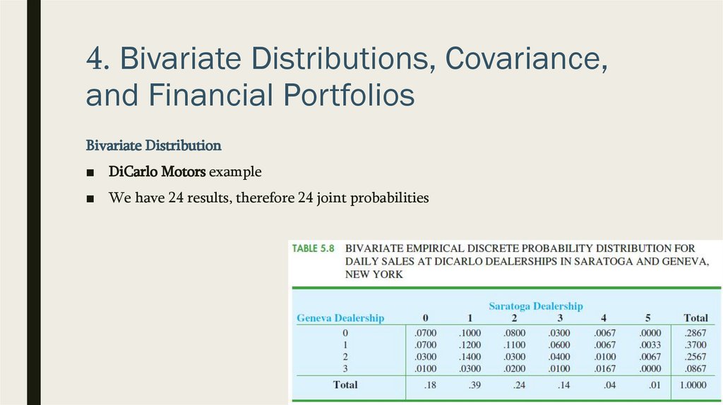
■ DiCarlo Motors example
■ We have 24 results, therefore 24 joint probabilities
36.
4. Bivariate Distributions, Covariance,and Financial Portfolios
Bivariate Distribution
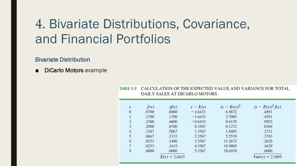
■ DiCarlo Motors example
■ We show the complete probability distribution for s = x + y along with the
computation of the expected value and variance
37.
4. Bivariate Distributions, Covariance,and Financial Portfolios
Bivariate Distribution
■ DiCarlo Motors example
38.
4. Bivariate Distributions, Covariance,and Financial Portfolios
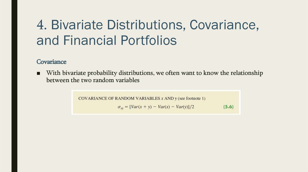
Covariance
■ With bivariate probability distributions, we often want to know the relationship
between the two random variables
39.
4. Bivariate Distributions, Covariance,and Financial Portfolios
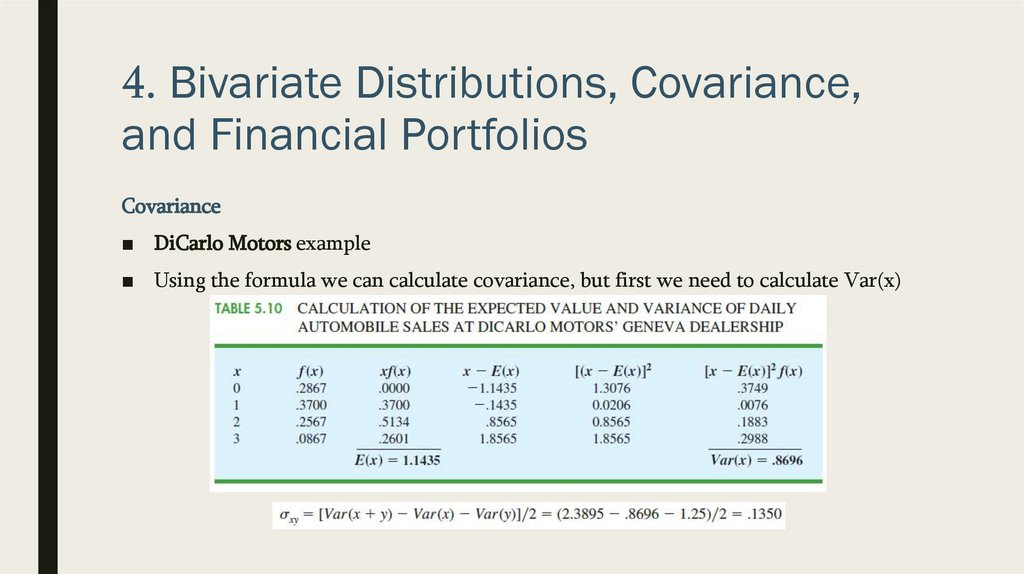
Covariance
■ DiCarlo Motors example
■ Using the formula we can calculate covariance, but first we need to calculate Var(x)
40.
4. Bivariate Distributions, Covariance,and Financial Portfolios
Covariance
■ DiCarlo Motors example
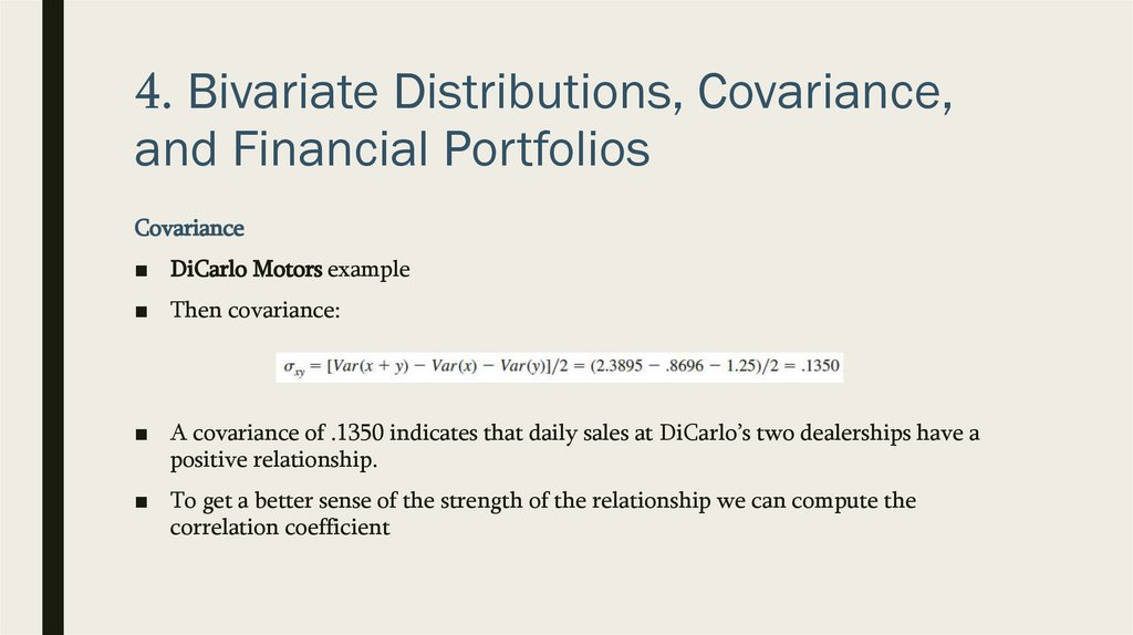
■ Then covariance:
■ A covariance of .1350 indicates that daily sales at DiCarlo’s two dealerships have a
positive relationship.
■ To get a better sense of the strength of the relationship we can compute the
correlation coefficient
41.
4. Bivariate Distributions, Covariance,and Financial Portfolios
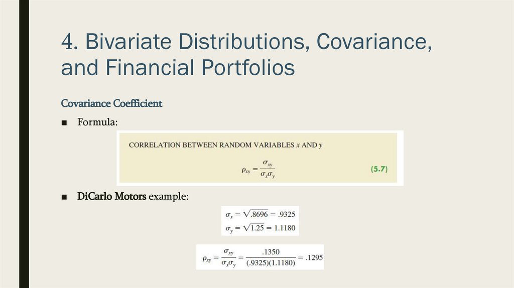
Covariance Coefficient
■ Formula:
■ DiCarlo Motors example:
42.
4. Bivariate Distributions, Covariance,and Financial Portfolios
Covariance Coefficient
■ DiCarlo Motors example
■ Covariance Coefficient is .1295
■ Correlation coefficient as a measure of the linear association between two variables
■ Values near +1 indicate a strong positive linear relationship; values near −1 indicate a
strong negative linear relationship; and values near zero indicate a lack of a linear
relationship
■ The correlation coefficient of .1295 indicates there is a weak positive relationship
between the random variables representing daily sales at the two DiCarlo dealerships
43.
4. Bivariate Distributions, Covariance,and Financial Portfolios
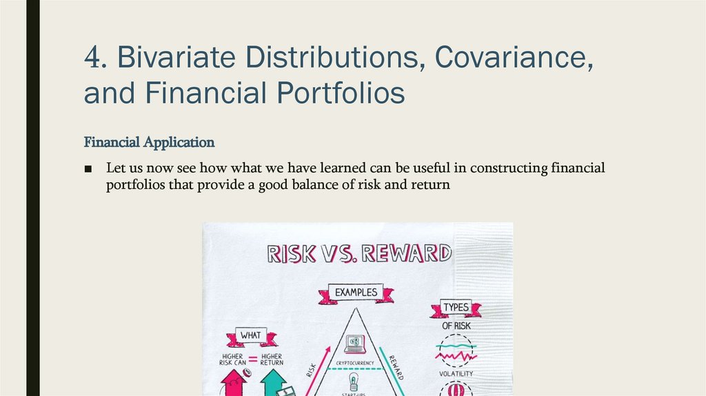
Financial Application
■ Let us now see how what we have learned can be useful in constructing financial
portfolios that provide a good balance of risk and return
44.
4. Bivariate Distributions, Covariance,and Financial Portfolios
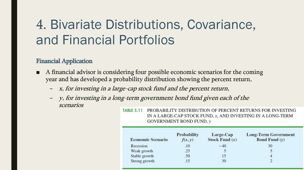
Financial Application
■ A financial advisor is considering four possible economic scenarios for the coming
year and has developed a probability distribution showing the percent return,
– x, for investing in a large-cap stock fund and the percent return,
– y, for investing in a long-term government bond fund given each of the
scenarios
45.
4. Bivariate Distributions, Covariance,and Financial Portfolios
Financial Application
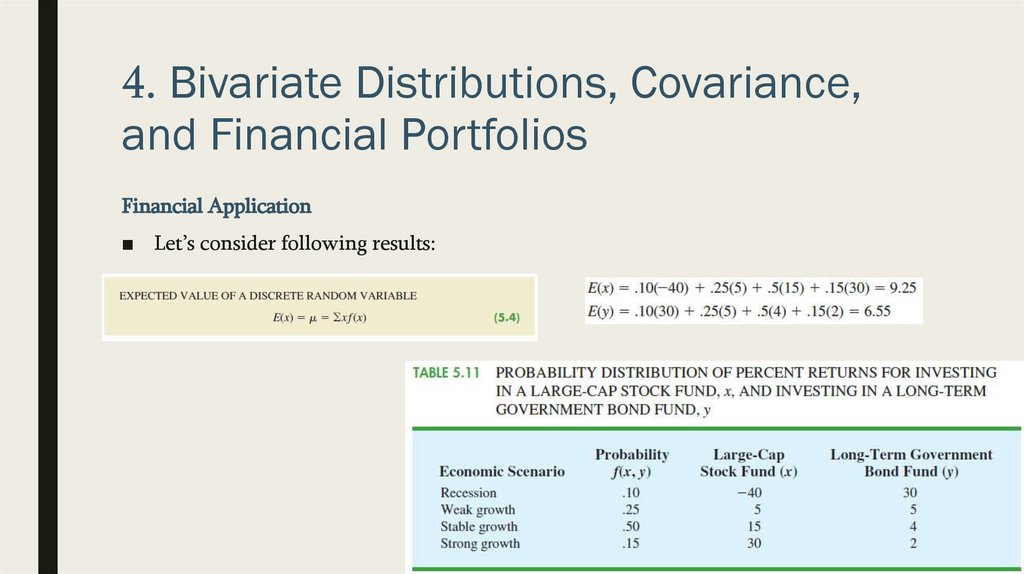
■ Let’s consider following results:
46.
4. Bivariate Distributions, Covariance,and Financial Portfolios
Financial Application
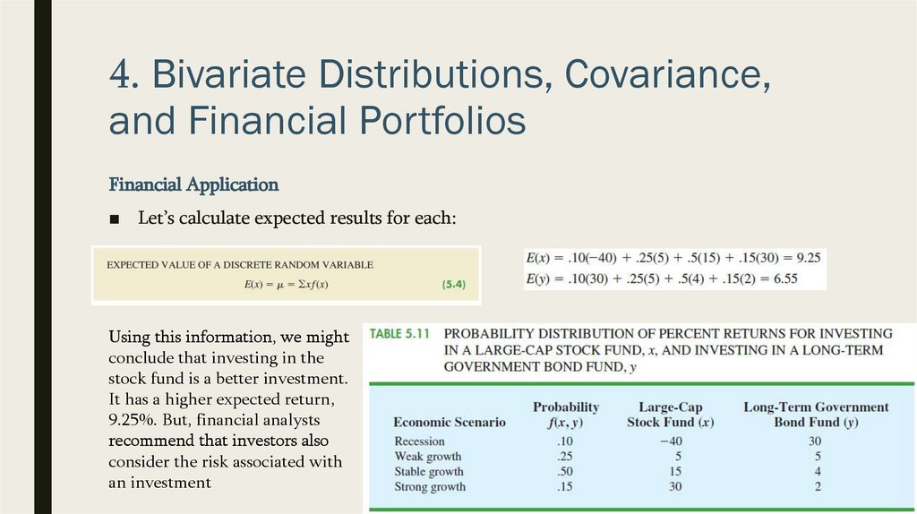
■ Let’s calculate expected results for each:
Using this information, we might
conclude that investing in the
stock fund is a better investment.
It has a higher expected return,
9.25%. But, financial analysts
recommend that investors also
consider the risk associated with
an investment
47.
4. Bivariate Distributions, Covariance,and Financial Portfolios
Financial Application
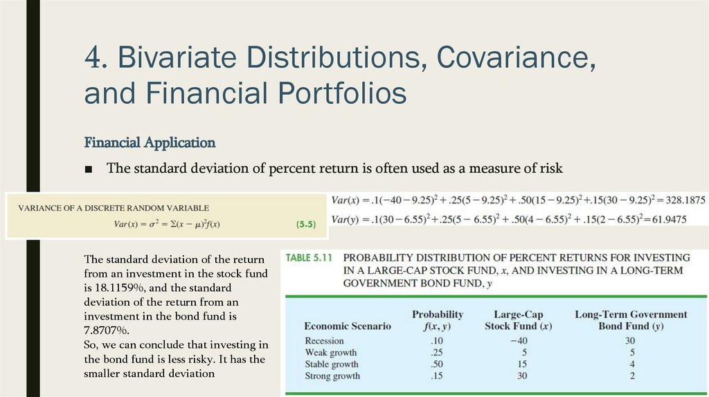
■ The standard deviation of percent return is often used as a measure of risk
The standard deviation of the return
from an investment in the stock fund
is 18.1159%, and the standard
deviation of the return from an
investment in the bond fund is
7.8707%.
So, we can conclude that investing in
the bond fund is less risky. It has the
smaller standard deviation
48.
4. Bivariate Distributions, Covariance,and Financial Portfolios
Financial Application
■
Investing in stocks has high return, but high risk; Investing in bonds has low return- low risk
■
An aggressive investor might choose the stock fund because of the higher expected return; a
conservative investor might choose the bond fund because of the lower risk. But, there are
other options. what about the possibility of investing in a portfolio consisting of both an
investment in the stock fund and an investment in the bond fund?
49.
4. Bivariate Distributions, Covariance,and Financial Portfolios
Financial Application
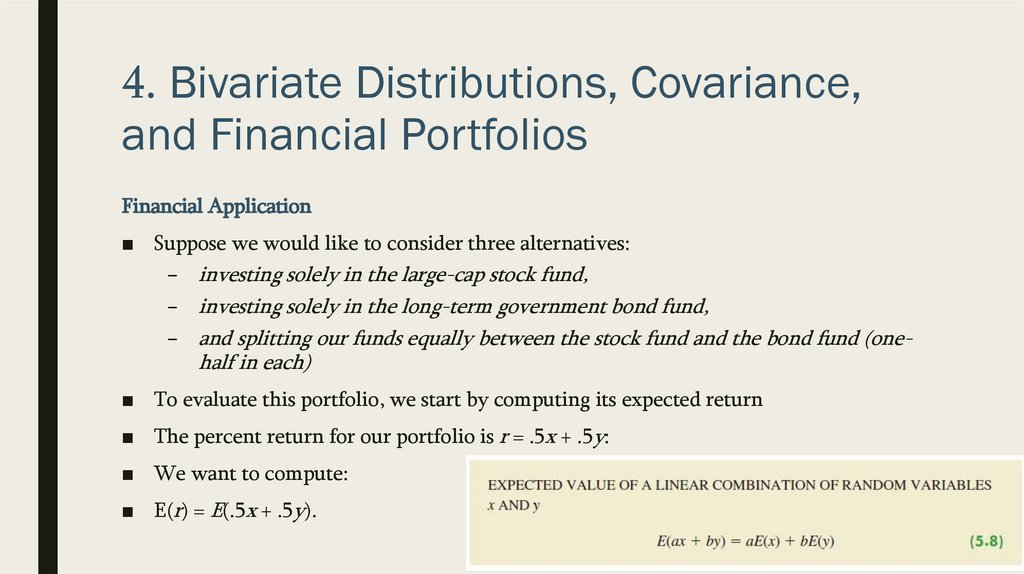
■ Suppose we would like to consider three alternatives:
– investing solely in the large-cap stock fund,
– investing solely in the long-term government bond fund,
– and splitting our funds equally between the stock fund and the bond fund (one-
half in each)
■ To evaluate this portfolio, we start by computing its expected return
■ The percent return for our portfolio is r = .5x + .5y:
■ We want to compute:
■ E(r) = E(.5x + .5y).
50.
4. Bivariate Distributions, Covariance,and Financial Portfolios
Financial Application
■ Since we have already computed E(x) = 9.25 and E(y) = 6.55, we can compute the
expected value of our portfolio:
■ E(.5x + .5y) = .5E(x) + .5E(y) = .5(9.25) + .5(6.55) = 7.9
■ We see that the expected return for investing in the portfolio is 7.9%.
■ With $100 invested, we would expect a return of $100(.079) = $7.90; with $1000
invested we would expect a return of $1000(.079) = $79.00; and so on.
■ But, what about the risk? As mentioned previously, financial analysts often use the
standard deviation as a measure of risk
51.
4. Bivariate Distributions, Covariance,and Financial Portfolios
Financial Application
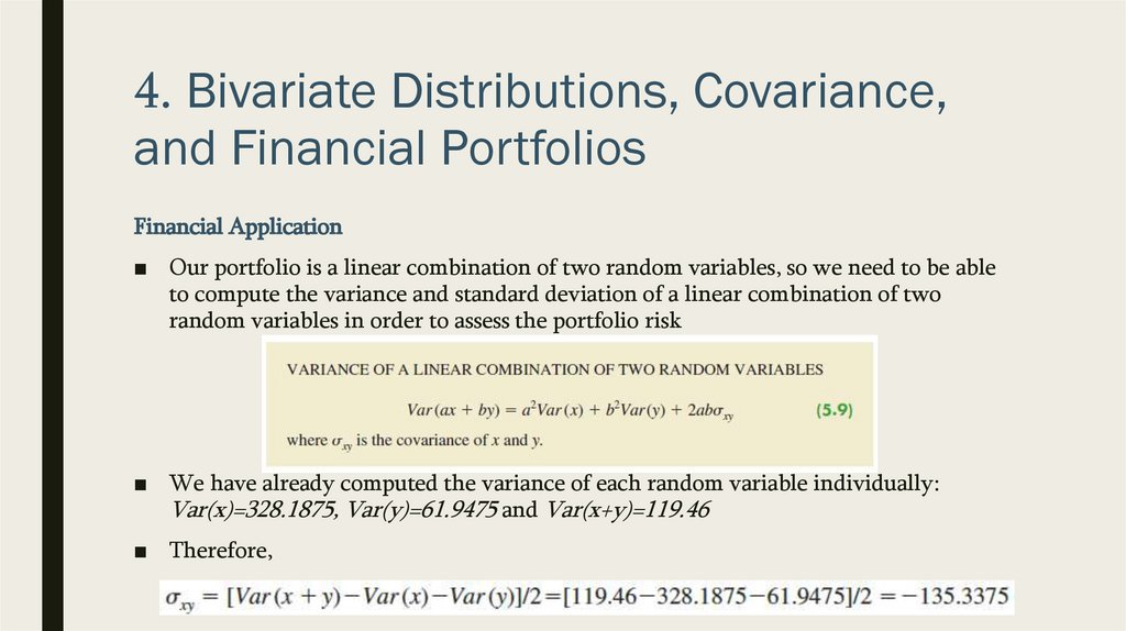
■ Our portfolio is a linear combination of two random variables, so we need to be able
to compute the variance and standard deviation of a linear combination of two
random variables in order to assess the portfolio risk
■ We have already computed the variance of each random variable individually:
Var(x)=328.1875, Var(y)=61.9475 and Var(x+y)=119.46
■ Therefore,
52.
4. Bivariate Distributions, Covariance,and Financial Portfolios
Financial Application
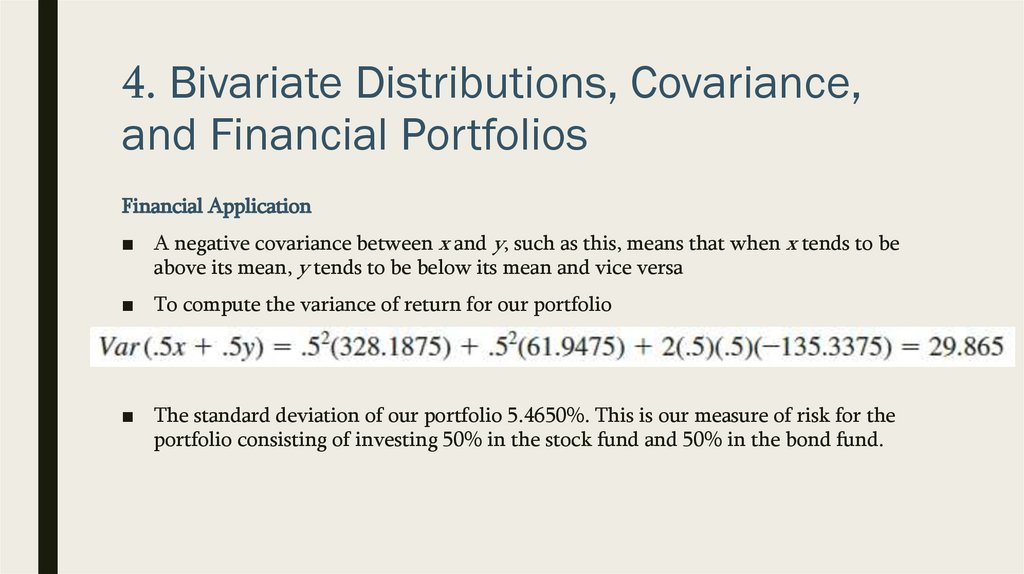
■ A negative covariance between x and y, such as this, means that when x tends to be
above its mean, y tends to be below its mean and vice versa
■ To compute the variance of return for our portfolio
■ The standard deviation of our portfolio 5.4650%. This is our measure of risk for the
portfolio consisting of investing 50% in the stock fund and 50% in the bond fund.
53.
4. Bivariate Distributions, Covariance,and Financial Portfolios
Financial Application
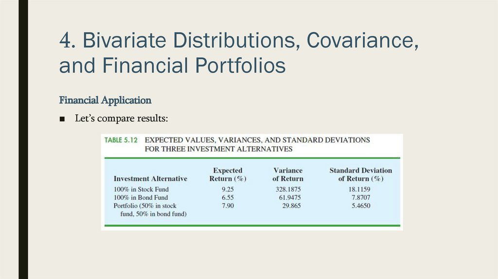
■ Let’s compare results:
54.
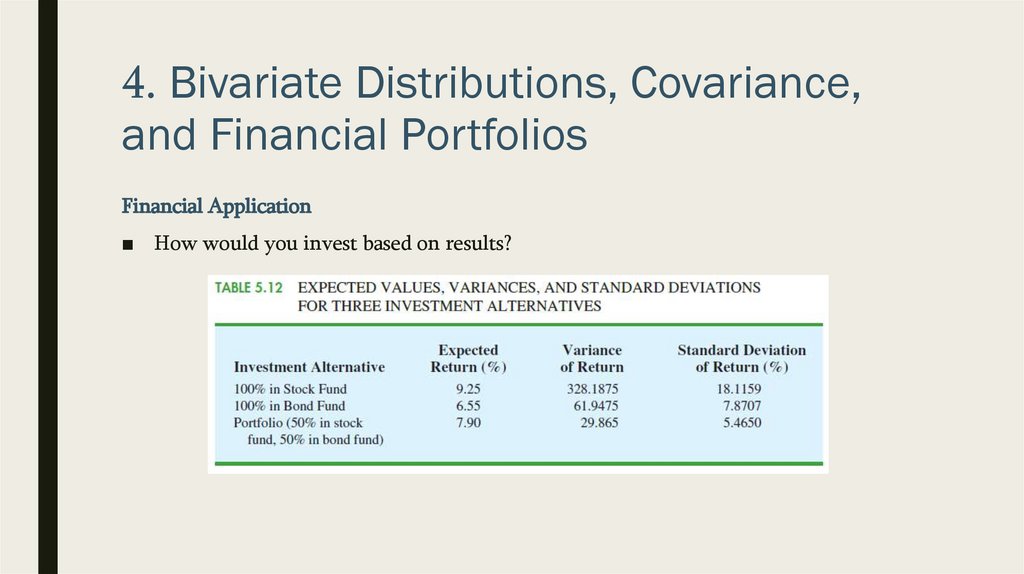
4. Bivariate Distributions, Covariance,and Financial Portfolios
Financial Application
■ How would you invest based on results?
55.
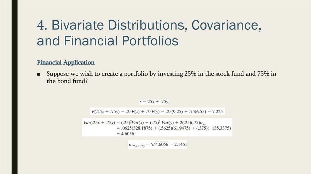
4. Bivariate Distributions, Covariance,and Financial Portfolios
Financial Application
■ Suppose we wish to create a portfolio by investing 25% in the stock fund and 75% in
the bond fund?
56.
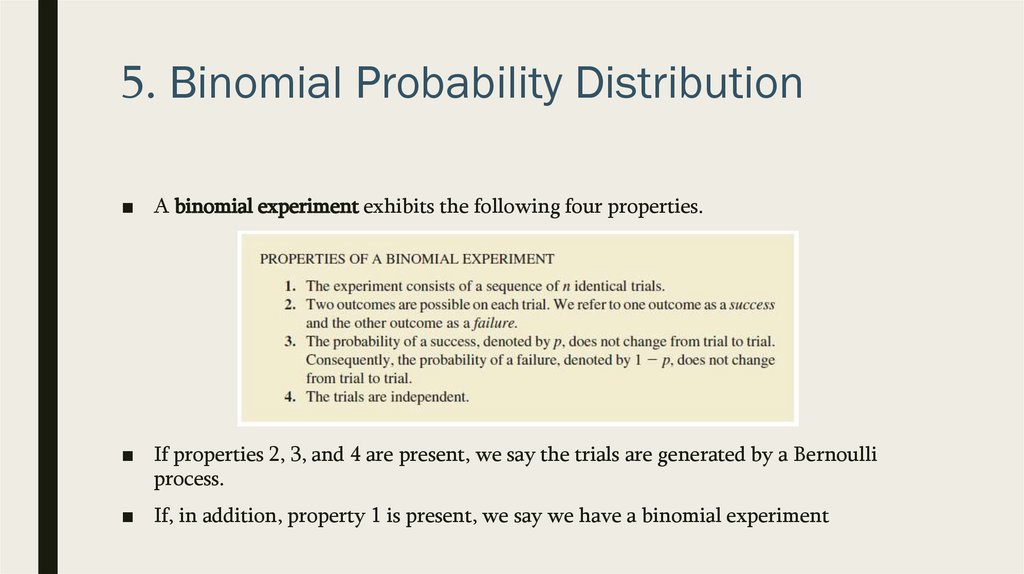
5. Binomial Probability Distribution■ A binomial experiment exhibits the following four properties.
■ If properties 2, 3, and 4 are present, we say the trials are generated by a Bernoulli
process.
■ If, in addition, property 1 is present, we say we have a binomial experiment
57.
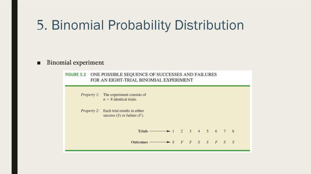
5. Binomial Probability Distribution■ Binomial experiment
58.
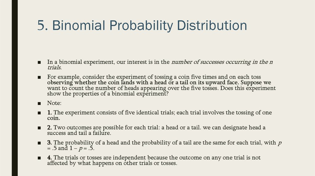
5. Binomial Probability Distribution■ In a binomial experiment, our interest is in the number of successes occurring in the n
trials.
■ For example, consider the experiment of tossing a coin five times and on each toss
observing whether the coin lands with a head or a tail on its upward face. Suppose we
want to count the number of heads appearing over the five tosses. Does this experiment
show the properties of a binomial experiment?
■ Note:
■ 1. The experiment consists of five identical trials; each trial involves the tossing of one
coin.
■ 2. Two outcomes are possible for each trial: a head or a tail. we can designate head a
success and tail a failure.
■ 3. The probability of a head and the probability of a tail are the same for each trial, with p
= .5 and 1 − p = .5.
■ 4. The trials or tosses are independent because the outcome on any one trial is not
affected by what happens on other trials or tosses.
59.
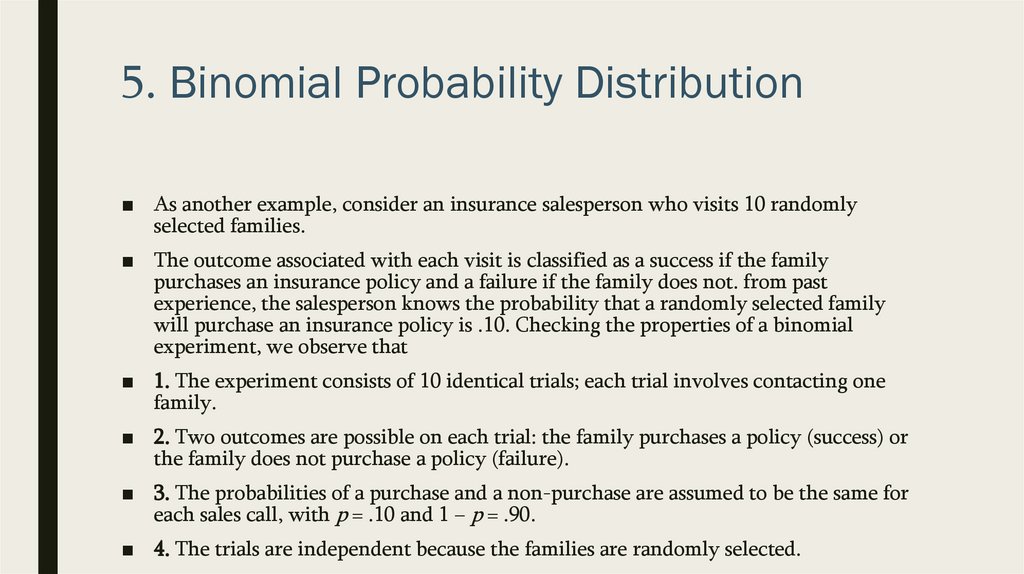
5. Binomial Probability Distribution■ As another example, consider an insurance salesperson who visits 10 randomly
selected families.
■ The outcome associated with each visit is classified as a success if the family
purchases an insurance policy and a failure if the family does not. from past
experience, the salesperson knows the probability that a randomly selected family
will purchase an insurance policy is .10. Checking the properties of a binomial
experiment, we observe that
■ 1. The experiment consists of 10 identical trials; each trial involves contacting one
family.
■ 2. Two outcomes are possible on each trial: the family purchases a policy (success) or
the family does not purchase a policy (failure).
■ 3. The probabilities of a purchase and a non-purchase are assumed to be the same for
each sales call, with p = .10 and 1 − p = .90.
■ 4. The trials are independent because the families are randomly selected.
60.
5. Binomial Probability Distribution■ Let’s consider practical example
61.
5. Binomial Probability DistributionMartin Clothing Store
■ Let us consider the purchase decisions of the next three customers who enter the
Martin Clothing Store
■ On the basis of past experience, the store manager estimates the probability that any
one customer will make a purchase is .30. what is the probability that two of the
next three customers will make a purchase?
■ Before we start analysis, let us verify that the experiment involving the sequence of
three purchase decisions can be viewed as a binomial experiment. Checking the four
requirements for a binomial experiment?
62.
5. Binomial Probability DistributionMartin Clothing Store
■ Using S to denote success (a
purchase) and F to denote failure
(no purchase), we are interested in
experimental outcomes involving
two successes in the three trials
(purchase decisions).
63.
5. Binomial Probability DistributionMartin Clothing Store
■ The number of experimental outcomes resulting in exactly x successes in n trials can
be computed using the following formula:
64.
5. Binomial Probability DistributionMartin Clothing Store
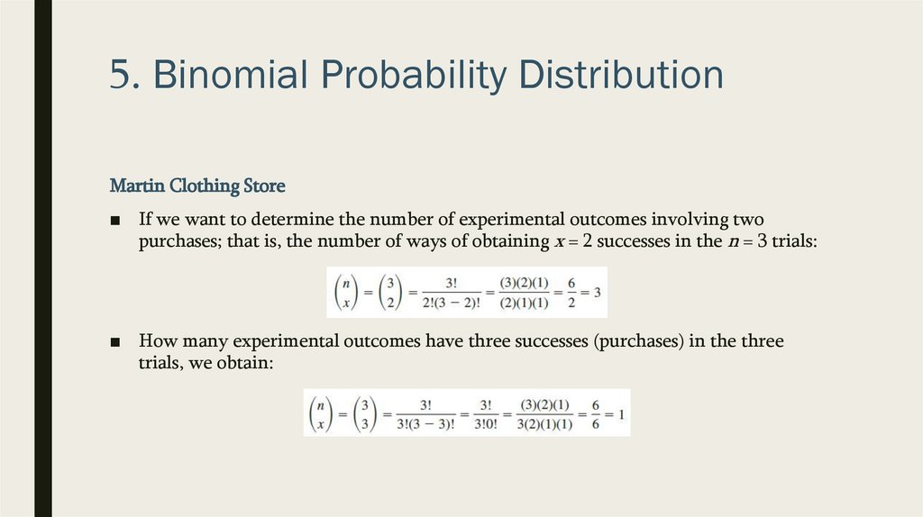
■ If we want to determine the number of experimental outcomes involving two
purchases; that is, the number of ways of obtaining x = 2 successes in the n = 3 trials:
■ How many experimental outcomes have three successes (purchases) in the three
trials, we obtain:
65.
5. Binomial Probability DistributionMartin Clothing Store
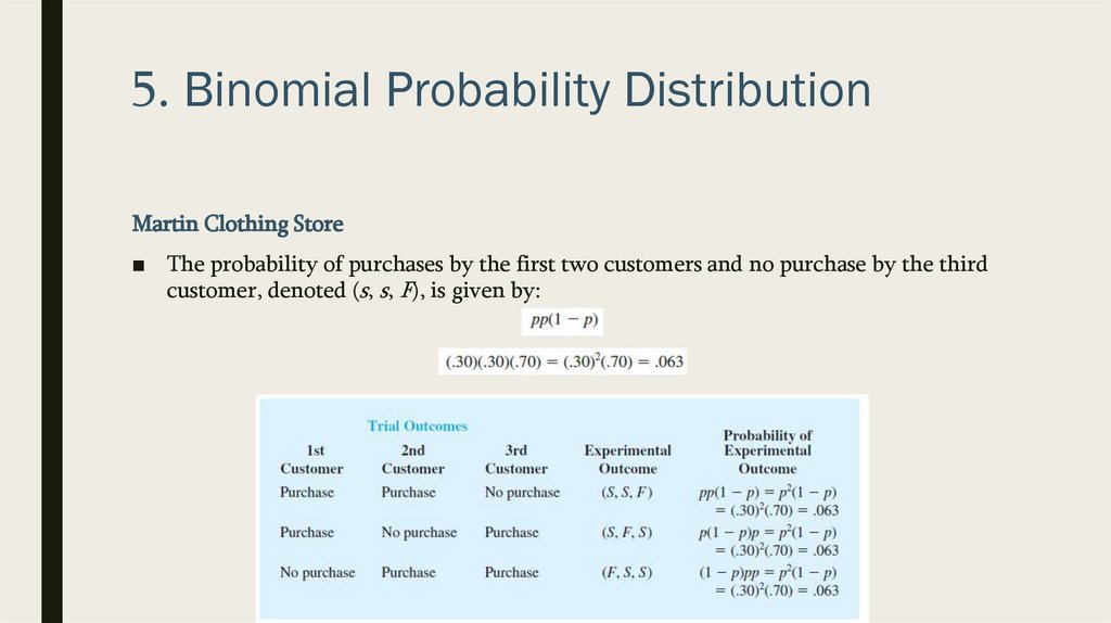
■ The probability of purchases by the first two customers and no purchase by the third
customer, denoted (s, s, F), is given by:
66.
5. Binomial Probability DistributionMartin Clothing Store
■ The formula shows that any experimental outcome with two successes has a
probability of .063
67.
5. Binomial Probability DistributionMartin Clothing Store
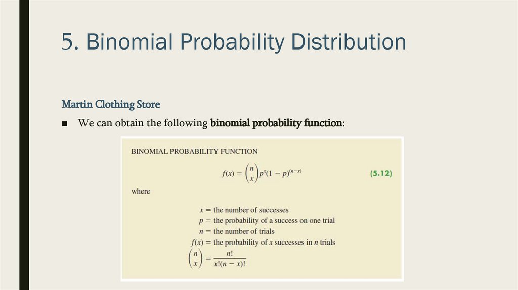
■ We can obtain the following binomial probability function:
68.
5. Binomial Probability DistributionMartin Clothing Store
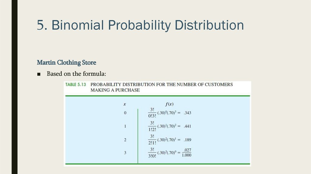
■ Based on the formula:
69.
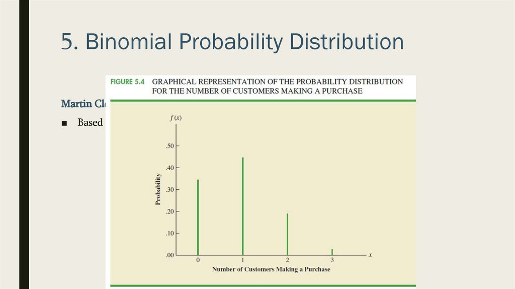
5. Binomial Probability DistributionMartin Clothing Store
■ Based on the formula:
70.
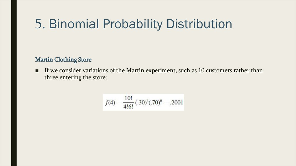
5. Binomial Probability DistributionMartin Clothing Store
■ If we consider variations of the Martin experiment, such as 10 customers rather than
three entering the store:
71.
5. Binomial Probability DistributionTables of Binomial Probabilities
■ We see that the probability
of x = 3 successes in a
binomial experiment with n
= 10 and p = .40 is .2150
72.
5. Binomial Probability DistributionExpected Value and Variance for the Binomial Distribution
■ Defined by formula:
■ Martin Clothing Store forecasts that 1000 customers will enter the store:
73.
5. Binomial Probability DistributionExpected Value and Variance for the Binomial Distribution
74.
6. Poisson Probability Distribution■ In this section we consider a discrete random variable that is often useful in
estimating the number of occurrences over a specified interval of time or space
■ For example,
■ the random variable of interest might be the number of arrivals at a car wash in one
hour, the number of repairs needed in 10 miles of highway, or the number of leaks
in 100 miles of pipeline.
75.
6. Poisson Probability Distribution■ Two properties
– The probability of an occurrence is the same for any two intervals of equal
length.
– The occurrence or nonoccurrence in any interval is independent of the
occurrence or nonoccurrence in any other interval
■ Formula
76.
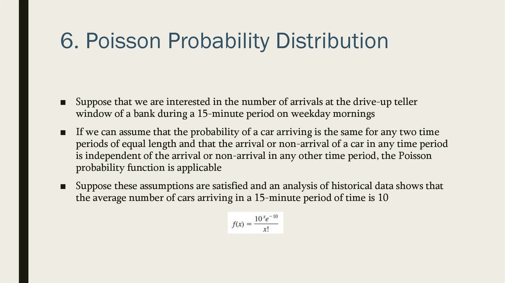
6. Poisson Probability Distribution■ Suppose that we are interested in the number of arrivals at the drive-up teller
window of a bank during a 15-minute period on weekday mornings
■ If we can assume that the probability of a car arriving is the same for any two time
periods of equal length and that the arrival or non-arrival of a car in any time period
is independent of the arrival or non-arrival in any other time period, the Poisson
probability function is applicable
■ Suppose these assumptions are satisfied and an analysis of historical data shows that
the average number of cars arriving in a 15-minute period of time is 10
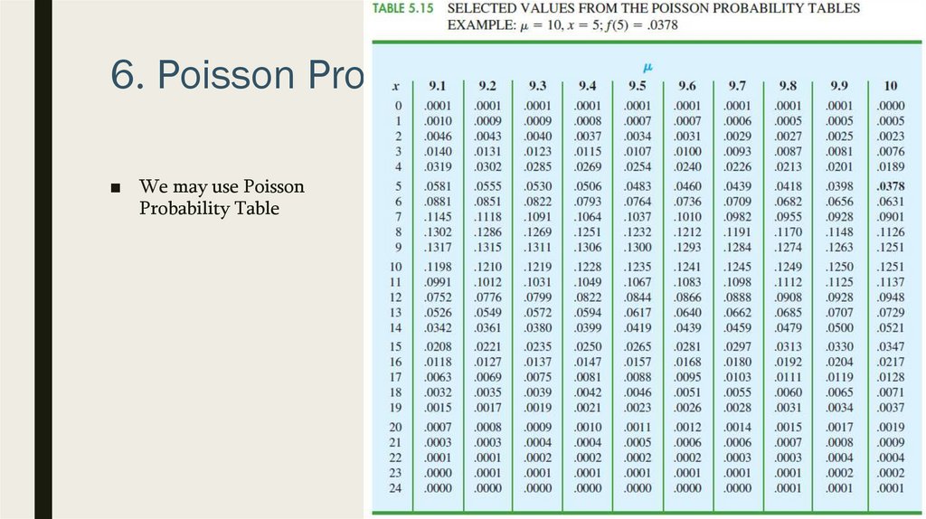
77.
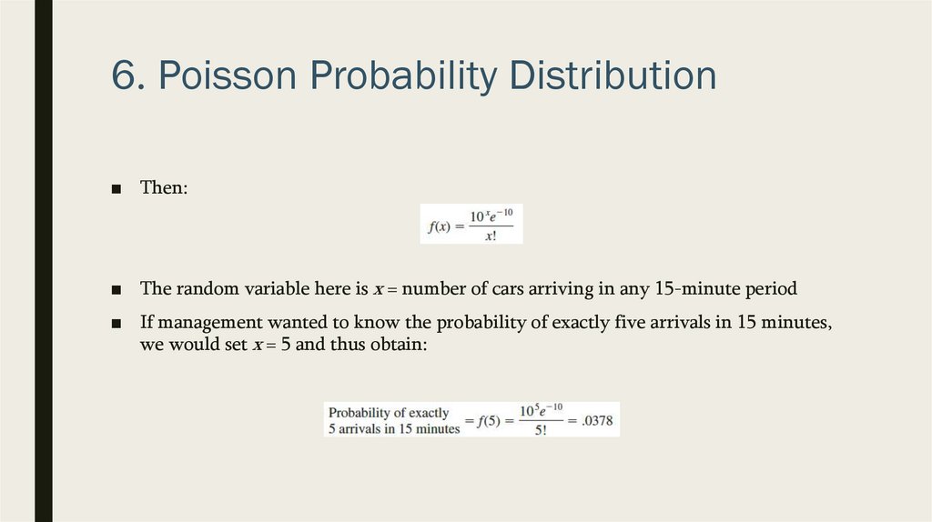
6. Poisson Probability Distribution■ Then:
■ The random variable here is x = number of cars arriving in any 15-minute period
■ If management wanted to know the probability of exactly five arrivals in 15 minutes,
we would set x = 5 and thus obtain:
78.
6. Poisson Probability Distribution■ We may use Poisson
Probability Table
79.
6. Hypergeometric ProbabilityDistribution
■ The hypergeometric probability distribution is closely related to the binomial
distribution.
■ The two probability distributions differ in two key ways.
– With the hypergeometric distribution, the trials are not independent;
– and the probability of success changes from trial to trial
80.
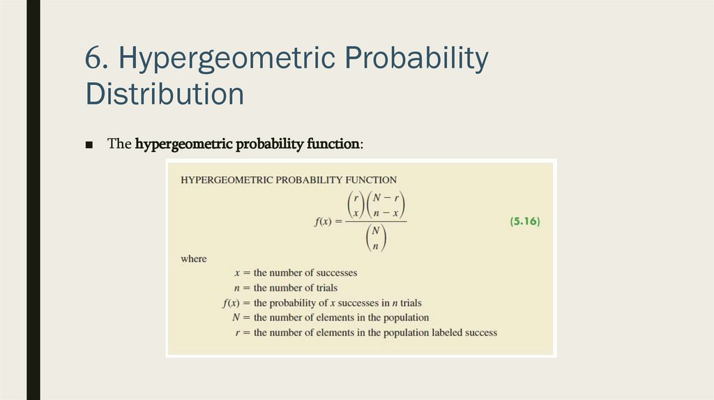
6. Hypergeometric ProbabilityDistribution
■ The hypergeometric probability function:
81.
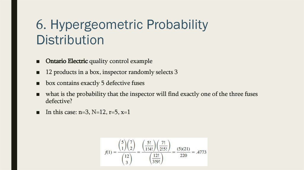
6. Hypergeometric ProbabilityDistribution
■ Ontario Electric quality control example
■ 12 products in a box, inspector randomly selects 3
■ box contains exactly 5 defective fuses
■ what is the probability that the inspector will find exactly one of the three fuses
defective?
■ In this case: n=3, N=12, r=5, x=1
82.
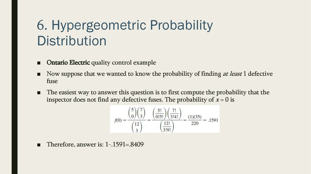
6. Hypergeometric ProbabilityDistribution
■ Ontario Electric quality control example
■ Now suppose that we wanted to know the probability of finding at least 1 defective
fuse
■ The easiest way to answer this question is to first compute the probability that the
inspector does not find any defective fuses. The probability of x = 0 is
■ Therefore, answer is: 1-.1591=.8409
83.
6. Hypergeometric ProbabilityDistribution
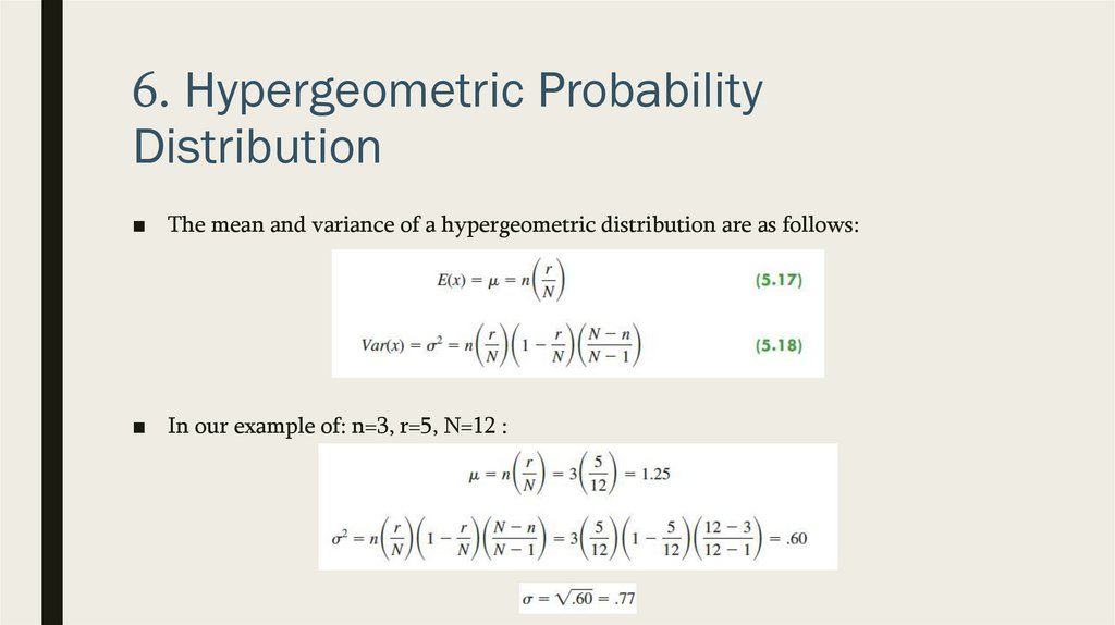
■ The mean and variance of a hypergeometric distribution are as follows:
■ In our example of: n=3, r=5, N=12 :