Probability Distributions

1. Probability Distributions

2. Random Variable

• A random variable x takes on a defined set of
values with different probabilities.
• For example, if you roll a die, the outcome is random
(not fixed) and there are 6 possible outcomes, each of
which occur with probability one-sixth.
• For example, if you poll people about their voting
preferences, the percentage of the sample that responds
“Yes on Proposition 100” is a also a random variable (the
percentage will be slightly differently every time you
poll).
• Roughly, probability is how frequently we
expect different outcomes to occur if we
repeat the experiment over and over
(“frequentist” view)

3. Random variables can be discrete or continuous

Discrete random variables have a
countable number of outcomes
Examples: Dead/alive, treatment/placebo,
dice, counts, etc.
Continuous random variables have an
infinite continuum of possible values.
Examples: blood pressure, weight, the
speed of a car, the real numbers from 1 to
6.

4. Probability functions

A probability function maps the possible
values of x against their respective
probabilities of occurrence, p(x)
p(x) is a number from 0 to 1.0.
The area under a probability function is
always 1.

5. Discrete example: roll of a die

p(x)
1/6
1
2
3
4
5
6
P(x) 1
all x
x

6. Probability mass function (pmf)

x
p(x)
1
p(x=1)=1/6
2
p(x=2)=1/6
3
p(x=3)=1/6
4
p(x=4)=1/6
5
p(x=5)=1/6
6
p(x=6)=1/6
1.0

7. Cumulative distribution function (CDF)

1.0
5/6
2/3
1/2
1/3
1/6
P(x)
1
2
3
4
5
6
x

8. Cumulative distribution function

x
P(x≤A)
1
P(x≤1)=1/6
2
P(x≤2)=2/6
3
P(x≤3)=3/6
4
P(x≤4)=4/6
5
P(x≤5)=5/6
6
P(x≤6)=6/6

9. Examples

1. What’s the probability that you roll a 3 or less?
P(x≤3)=1/2
2. What’s the probability that you roll a 5 or higher?
P(x≥5) = 1 – P(x≤4) = 1-2/3 = 1/3

10. Practice Problem

Which of the following are probability functions?
a.
f(x)=.25 for x=9,10,11,12
b.
f(x)= (3-x)/2 for x=1,2,3,4
c.
f(x)= (x2+x+1)/25 for x=0,1,2,3

11. Answer (a)

a.
f(x)=.25 for x=9,10,11,12
x
f(x)
9
.25
10
.25
11
.25
12
.25
1.0
Yes, probability
function!

12. Answer (b)

b.
f(x)= (3-x)/2 for x=1,2,3,4
x
f(x)
1
(3-1)/2=1.0
2
(3-2)/2=.5
3
(3-3)/2=0
4
(3-4)/2=-.5
Though this sums to 1,
you can’t have a negative
probability; therefore, it’s
not a probability
function.

13. Answer (c)

f(x)= (x2+x+1)/25 for x=0,1,2,3
c.
x
f(x)
0
1/25
1
3/25
2
7/25
3
13/25
24/25
Doesn’t sum to 1. Thus,
it’s not a probability
function.

14. Practice Problem:

The number of ships to arrive at a harbor on any given day is a
random variable represented by x. The probability distribution
for x is:
x
P(x)
10
.4
11
.2
12
.2
13
.1
14
.1
Find the probability that on a given day:
a.
exactly 14 ships arrive
b.
At least 12 ships arrive
p(x 12)= (.2 + .1 +.1) = .4
c.
At most 11 ships arrive
p(x≤11)= (.4 +.2) = .6
p(x=14)= .1

15. Practice Problem:

You are lecturing to a group of 1000 students. You
ask them to each randomly pick an integer between
1 and 10. Assuming, their picks are truly random:
What’s your best guess for how many students picked
the number 9?
Since p(x=9) = 1/10, we’d expect about 1/10th of the 1000
students to pick 9. 100 students.
What percentage of the students would you expect
picked a number less than or equal to 6?
Since p(x≤ 6) = 1/10 + 1/10 + 1/10 + 1/10 + 1/10 + 1/10 =.6
60%

16. Important discrete distributions in epidemiology…

Binomial
Yes/no outcomes (dead/alive,
treated/untreated, smoker/non-smoker,
sick/well, etc.)
Poisson
Counts (e.g., how many cases of disease in
a given area)

17. Continuous case

The probability function that accompanies a
continuous random variable is a continuous
mathematical function that integrates to 1.
The probabilities associated with continuous
functions are just areas under the curve (integrals!).
Probabilities are given for a range of values, rather
than a particular value (e.g., the probability of
getting a math SAT score between 700 and 800 is
2%).

18. Continuous case

For example, recall the negative exponential
function (in probability, this is called an
“exponential distribution”):
f ( x) e x
This function integrates to 1:
e
0
x
e
x
0
0 1 1

19. Continuous case: “probability density function” (pdf)

p(x)=e-x
1
x
The probability that x is any exact particular value (such as 1.9976) is 0;
we can only assign probabilities to possible ranges of x.

20.

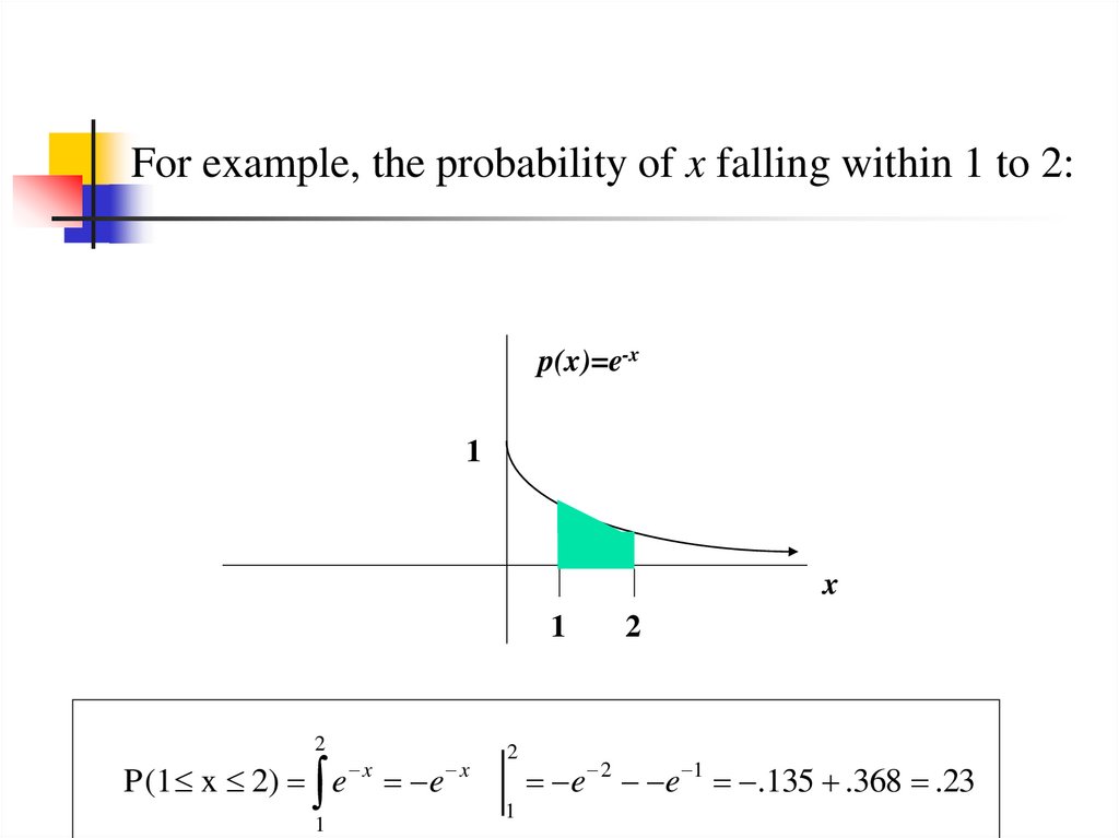
For example, the probability of x falling within 1 to 2:
p(x)=e-x
1
x
1
2
P(1 x 2) e
1
x
e
x
2
1
2
e 2 e 1 .135 .368 .23

21. Cumulative distribution function

As in the discrete case, we can specify the “cumulative
distribution function” (CDF):
The CDF here = P(x≤A)=
A
0
e
x
e
x
A
0
e A e 0 e A 1 1 e A

22. Example

p(x)
1
2
P(x 2) 1 - e
2
x
1 - .135 .865

23. Example 2: Uniform distribution

The uniform distribution: all values are equally likely
The uniform distribution:
f(x)= 1 , for 1 x 0
p(x)
1
x
1
We can see it’s a probability distribution because it integrates
to 1 (the area under the curve is 1):
1
1
1 x
0
1 0 1
0

24. Example: Uniform distribution

What’s the probability that x is between ¼ and ½?
p(x)
1
¼ ½
P(½ x ¼ )= ¼
1
x

25. Practice Problem

4. Suppose that survival drops off rapidly in the year following diagnosis of a
certain type of advanced cancer. Suppose that the length of survival (or
time-to-death) is a random variable that approximately follows an
exponential distribution with parameter 2 (makes it a steeper drop off):
probabilit y function : p( x T ) 2e 2T
[note : 2e
0
2 x
e
2 x
0 1 1]
0
What’s the probability that a person who is diagnosed with this
illness survives a year?

26. Answer

The probability of dying within 1 year can be calculated using the cumulative
distribution function:
Cumulative distribution function is:
P ( x T ) e
2 x
T
1 e 2 (T )
0
The chance of surviving past 1 year is: P(x≥1) = 1 – P(x≤1)
1 (1 e 2(1) ) .135

27. Expected Value and Variance

All probability distributions are
characterized by an expected value and
a variance (standard deviation
squared).

28.

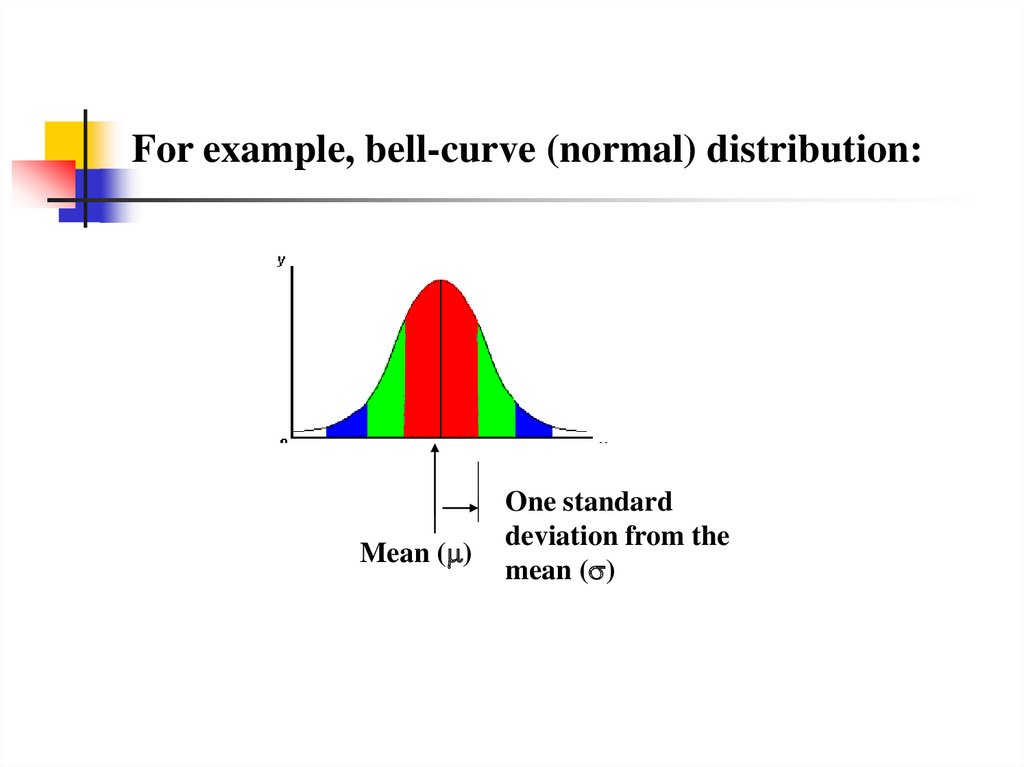
For example, bell-curve (normal) distribution:
Mean ( )
One standard
deviation from the
mean ( )

29. Expected value, or mean

If we understand the underlying probability function of a
certain phenomenon, then we can make informed
decisions based on how we expect x to behave on-average
over the long-run…(so called “frequentist” theory of
probability).
Expected value is just the weighted average or mean (µ)
of random variable x. Imagine placing the masses p(x) at
the points X on a beam; the balance point of the beam is
the expected value of x.

30. Example: expected value

Recall the following probability distribution of
ship arrivals:
x
P(x)
10
.4
5
11
.2
12
.2
13
.1
14
.1
x p( x) 10(.4) 11(.2) 12(.2) 13(.1) 14(.1) 11.3
i
i 1

31. Expected value, formally

Discrete case:
E( X )
x p(x )
i
i
all x
Continuous case:
E( X )
xi p(xi )dx
all x

32. Empirical Mean is a special case of Expected Value…

Sample mean, for a sample of n subjects: =
n
X
x
i 1
n
i
n
i 1
1
xi ( )
n
The probability (frequency) of each
person in the sample is 1/n.

33. Expected value, formally

Discrete case:
E( X )
x p(x )
i
i
all x
Continuous case:
E( X )
xi p(xi )dx
all x

34. Extension to continuous case: uniform distribution

p(x)
1
x
1
1
x2
E ( X ) x(1)dx
2
0
1
0
1
1
0
2
2

35. Symbol Interlude

E(X) = µ
these symbols are used interchangeably

36. Expected Value

Expected value is an extremely useful
concept for good decision-making!

37. Example: the lottery

The Lottery (also known as a tax on people
who are bad at math…)
A certain lottery works by picking 6 numbers
from 1 to 49. It costs $1.00 to play the
lottery, and if you win, you win $2 million
after taxes.
If you play the lottery once, what are your
expected winnings or losses?

38. Lottery

Calculate the probability of winning in 1 try:
1
49
6
“49 choose 6”
1
1
7.2 x 10 -8
49! 13,983,816
43!6!
Out of 49 numbers,
this is the number
of distinct
combinations of 6.
The probability function (note, sums to 1.0):
x$
p(x)
-1
.999999928
+ 2 million
7.2 x 10--8

39. Expected Value

The probability function
x$
p(x)
-1
.999999928
+ 2 million
7.2 x 10--8
Expected Value
E(X) = P(win)*$2,000,000 + P(lose)*-$1.00
= 2.0 x 106 * 7.2 x 10-8+ .999999928 (-1) = .144 - .999999928 = -$.86
Negative expected value is never good!
You shouldn’t play if you expect to lose money!

40. Expected Value

If you play the lottery every week for 10 years, what are your
expected winnings or losses?
520 x (-.86) = -$447.20

41. Gambling (or how casinos can afford to give so many free drinks…)

A roulette wheel has the numbers 1 through 36, as well as 0 and 00.
If you bet $1 that an odd number comes up, you win or lose $1
according to whether or not that event occurs. If random variable X
denotes your net gain, X=1 with probability 18/38 and X= -1 with
probability 20/38.
E(X) = 1(18/38) – 1 (20/38) = -$.053
On average, the casino wins (and the player loses) 5 cents per game.
The casino rakes in even more if the stakes are higher:
E(X) = 10(18/38) – 10 (20/38) = -$.53
If the cost is $10 per game, the casino wins an average of 53 cents per
game. If 10,000 games are played in a night, that’s a cool $5300.

42. **A few notes about Expected Value as a mathematical operator:

If c= a constant number (i.e., not a variable) and X and Y are any
random variables…
E(c) = c
E(cX)=cE(X)
E(c + X)=c + E(X)
E(X+Y)= E(X) + E(Y)

43. E(c) = c

E(c) = c
Example: If you cash in soda cans in CA, you always get 5 cents
per can.
Therefore, there’s no randomness. You always expect to (and
do) get 5 cents.

44. E(cX)=cE(X)

E(cX)=cE(X)
Example: If the casino charges $10 per game instead of $1,
then the casino expects to make 10 times as much on average
from the game (See roulette example above!)

45. E(c + X)=c + E(X)

E(c + X)=c + E(X)
Example, if the casino throws in a free drink worth exactly $5.00
every time you play a game, you always expect to (and do) gain
an extra $5.00 regardless of the outcome of the game.

46. E(X+Y)= E(X) + E(Y)

E(X+Y)= E(X) + E(Y)
Example: If you play the lottery twice, you expect to lose: -$.86
+ -$.86.
NOTE: This works even if X and Y are dependent!! Does
not require independence!! Proof left for later…

47. Practice Problem

If a disease is fairly rare and the antibody test is fairly
expensive, in a resource-poor region, one strategy is to take
half of the serum from each sample and pool it with n other
halved samples, and test the pooled lot. If the pooled lot is
negative, this saves n-1 tests. If it’s positive, then you go
back and test each sample individually, requiring n+1 tests
total.
a.
b.
c.
Suppose a particular disease has a prevalence of 10% in a thirdworld population and you have 500 blood samples to screen. If
you pool 20 samples at a time (25 lots), how many tests do you
expect to have to run (assuming the test is perfect!)?
What if you pool only 10 samples at a time?
5 samples at a time?

48. Answer (a)

a. Suppose a particular disease has a prevalence of 10% in a third-world
population and you have 500 blood samples to screen. If you pool 20
samples at a time (25 lots), how many tests do you expect to have to
run (assuming the test is perfect!)?
Let X = a random variable that is the number of tests you have to run per
lot:
E(X) = P(pooled lot is negative)(1) + P(pooled lot is positive) (21)
E(X) = (.90)20 (1) + [1-.9020] (21)
18.56
= 12.2% (1) + 87.8% (21) =
E(total number of tests) = 25*18.56 = 464

49. Answer (b)

b. What if you pool only 10 samples at a time?
E(X) = (.90)10 (1) + [1-.9010] (11)
average per lot
50 lots * 7.5 = 375
= 35% (1) + 65% (11) = 7.5

50. Answer (c)

c. 5 samples at a time?
E(X) = (.90)5 (1) + [1-.905] (6)
100 lots * 3.05 = 305
= 59% (1) + 41% (6) = 3.05 average per lot

51. Practice Problem

If X is a random integer between 1 and 10,
what’s the expected value of X?

52. Answer

If X is a random integer between 1 and 10, what’s the expected
value of X?
10
1
1
E ( x) i ( )
10
i 1 10
10
i
i (.1)
10(10 1)
55(.1) 5.5
2

53. Expected value isn’t everything though…

Take the show “Deal or No Deal”
Everyone know the rules?
Let’s say you are down to two cases left. $1
and $400,000. The banker offers you
$200,000.
So, Deal or No Deal?

54. Deal or No Deal…

This could really be represented as a
probability distribution and a nonrandom variable:
x$
p(x)
+1
.50
+$400,000
.50
x$
p(x)
+$200,000
1.0

55. Expected value doesn’t help…

x$
p(x)
+1
.50
+$400,000
.50
E( X )
x p(x ) 1(.50) 400,000(.50) 200,000
i
i
all x
x$
p(x)
+$200,000
1.0
E ( X ) 200,000

56. How to decide?

Variance!
• If you take the deal, the variance/standard
deviation is 0.
•If you don’t take the deal, what is average
deviation from the mean?
•What’s your gut guess?

57. Variance/standard deviation

“The average (expected) squared
distance (or deviation) from the mean”
Var ( x) E[( x ) ]
2
2
(x )
i
2
p(xi )
all x
**We square because squaring has better properties than
absolute value. Take square root to get back linear average
distance from the mean (=”standard deviation”).

58. Variance, formally

Discrete case:
Var ( X )
2
(x )
i
2
p(xi )
all x
Continuous case:
Var ( X ) ( xi ) p( xi )dx
2
2

59. Similarity to empirical variance

The variance of a sample: s2 =
N
( xi x ) 2
i 1
n 1
N
1
( xi x ) (
)
n 1
i 1
2
Division by n-1 reflects the fact that we have lost a
“degree of freedom” (piece of information) because
we had to estimate the sample mean before we could
estimate the sample variance.

60. Symbol Interlude

Var(X) = 2
these symbols are used interchangeably

61. Variance: Deal or No Deal

2
(x
) p(xi )
2
i
all x
2
( xi ) 2 p(xi )
all x
(1 200,000 ) 2 (.5) (400,000 200,000 ) 2 (.5) 200,000 2
200,000 2 200,000
Now you examine your personal risk tolerance…

62. Practice Problem

A roulette wheel has the numbers 1 through
36, as well as 0 and 00. If you bet $1.00 that
an odd number comes up, you win or lose
$1.00 according to whether or not that event
occurs. If X denotes your net gain, X=1 with
probability 18/38 and X= -1 with probability
20/38.
We already calculated the mean to be = -$.053.
What’s the variance of X?

63. Answer

2
(x )
2
i
p(xi )
all x
( 1 .053) 2 (18 / 38) ( 1 .053) 2 (20 / 38)
(1.053) 2 (18 / 38) ( 1 .053) 2 (20 / 38)
(1.053) 2 (18 / 38) ( .947) 2 (20 / 38)
.997
.997 .99
Standard deviation is $.99. Interpretation: On average, you’re
either 1 dollar above or 1 dollar below the mean, which is just
under zero. Makes sense!

64. Handy calculation formula!

Handy calculation formula (if you ever need to calculate by hand!):
Var ( X )
(x )
i
2
p(xi )
all x
x
i
2
p(xi ) ( )
2
all x
E ( x ) [ E ( x)]
2
Intervening algebra!
2

65. Var(x) = E(x-)2 = E(x2) – [E(x)]2 (your calculation formula!)

Var(x) = E(x- )2 = E(x2) – [E(x)]2
(your calculation formula!)
Proofs (optional!):
E(x- )2 = E(x2–2 x + 2)
=E(x2) – E(2 x) +E( 2)
= E(x2) – 2 E(x) + 2
= E(x2) – 2 + 2
= E(x2) – 2
= E(x2) – [E(x)]2
OR, equivalently:
E(x- )2 =
[( x )
allx
2
] p( x)
[( x
2
2 x 2 ] p( x)
allx
E ( x 2 ) 2 2 2 (1) E ( x 2 ) 2
remember “FOIL”?!
Use rules of expected value:E(X+Y)= E(X) + E(Y)
E(c) = c
E(x) =
x
allx
2
p ( x) 2
xp( x) p( x) E( x
2
2
) 2 E ( x) 2 (1)

66. For example, what’s the variance and standard deviation of the roll of a die?

1
x
p(x)
p(x=1)=1/6
2
p(x=2)=1/6
3
p(x=3)=1/6
4
p(x=4)=1/6
5
p(x=5)=1/6
6
p(x=6)=1/6
1.0
E ( x)
p(x)
average distance from the mean
1/
6
1 2 3 4 5 6
x
mean
1
1
1
1
1
1 21
xi p(xi ) (1)( ) 2( ) 3( ) 4( ) 5( ) 6( ) 3.5
6
6
6
6
6
6
6
all x
1
1
1
1
1
1
E( x )
xi p(xi ) (1)( ) 4( ) 9( ) 16( ) 25( ) 36( ) 15.17
6
6
6
6
6
6
all x
2
2
x2 Var( x) E ( x 2 ) [ E ( x)]2 15.17 3.52 2.92
x 2.92 1.71

67. **A few notes about Variance as a mathematical operator:

If c= a constant number (i.e., not a variable) and X and
Y are random variables, then
Var(c) = 0
Var (c+X)= Var(X)
Var(cX)= c2Var(X)
Var(X+Y)= Var(X) + Var(Y) ONLY IF X and
Y are independent!!!!
{Var(X+Y)= Var(X) + Var(Y)+2Cov(X,Y) IF X
and Y are not independent}

68. Var(c) = 0

Var(c) = 0
Constants don’t vary!

69. Var (c+X)= Var(X)

Var (c+X)= Var(X)
Adding a constant to every instance of a random variable
doesn’t change the variability. It just shifts the whole
distribution by c. If everybody grew 5 inches suddenly, the
variability in the population would still be the same.
+c

70. Var (c+X)= Var(X)

Var (c+X)= Var(X)
Adding a constant to every instance of a random variable
doesn’t change the variability. It just shifts the whole
distribution by c. If everybody grew 5 inches suddenly, the
variability in the population would still be the same.
+c

71. Var(cX)= c2Var(X)

Var(cX)=
2
c Var(X)
Var(cX)= c2Var(X)
Multiplying each instance of the random variable by c makes it
c-times as wide of a distribution, which corresponds to c2 as
much variance (deviation squared). For example, if everyone
suddenly became twice as tall, there’d be twice the deviation
and 4 times the variance in heights in the population.

72. Var(X+Y)= Var(X) + Var(Y)

Var(X+Y)= Var(X) + Var(Y) ONLY IF X and Y are
independent!!!!!!!!
With two random variables, you have more opportunity for
variation, unless they vary together (are dependent, or have
covariance): Var(X+Y)= Var(X) + Var(Y) + 2Cov(X, Y)

73. Example of Var(X+Y)= Var(X) + Var(Y): TPMT

TPMT metabolizes the drugs 6mercaptopurine, azathioprine, and 6thioguanine (chemotherapy drugs)
People with TPMT-/ TPMT+ have reduced
levels of activity (10% prevalence)
People with TPMT-/ TPMT- have no TPMT
activity (prevalence 0.3%).
They cannot metabolize 6mercaptopurine, azathioprine, and 6thioguanine, and risk bone marrow toxicity if
given these drugs.

74. TPMT activity by genotype

Weinshilboum R. Drug Metab Dispos. 2001 Apr;29(4 Pt 2):601-5

75. TPMT activity by genotype

The variability in TPMT
activity is much higher
in wild-types than
heterozygotes.
Weinshilboum R. Drug Metab Dispos. 2001 Apr;29(4 Pt 2):601-5

76. TPMT activity by genotype

No variability in
expression here,
since there’s no
working gene.
There is variability in
expression from each
wild-type allele. With
two copies of the
good gene present,
there’s “twice as
much” variability.
Weinshilboum R. Drug Metab Dispos. 2001 Apr;29(4 Pt 2):601-5

77. Practice Problem

Find the variance and standard deviation for the
number of ships to arrive at the harbor (recall
that the mean is 11.3).
x
P(x)
10
.4
11
.2
12
.2
13
.1
14
.1

78. Answer: variance and std dev

x2
P(x)
E(x 2 )
5
100
.4
121
.2
144
.2
169
.1
196
.1
xi p ( x i ) (100 )(.4) (121)(.2) 144 (.2) 169 (.1) 196 (.1) 129 .5
2
i 1
Var( x) E ( x 2 ) [ E ( x)] 2 129 .5 11.3 2 1.81
stddev( x) 1.81 1.35
Interpretation: On an average day, we expect 11.3 ships to
arrive in the harbor, plus or minus 1.35. This gives you a feel
for what would be considered a usual day!

79. Practice Problem

You toss a coin 100 times. What’s the expected number of
heads? What’s the variance of the number of heads?

80. Answer: expected value

Intuitively, we’d probably all agree that we expect around 50 heads, right?
Another way to show this
Think of tossing 1 coin. E(X=number of heads) = (1) P(heads) + (0)P(tails)
E(X=number of heads) = 1(.5) + 0 = .5
If we do this 100 times, we’re looking for the sum of 100 tosses, where we
assign 1 for a heads and 0 for a tails. (these are 100 “independent, identically
distributed (i.i.d)” events)
E(X1 +X2 +X3 +X4 +X5 …..+X100) = E(X1) + E(X2) + E(X3)+ E(X4)+ E(X5) …..+
E(X100) =
100 E(X1) = 50

81. Answer: variance

What’s the variability, though? More tricky. But, again, we could do
this for 1 coin and then use our rules of variance.
Think of tossing 1 coin.
E(X2=number of heads squared) = 12 P(heads) + 02 P(tails)
E(X2) = 1(.5) + 0 = .5
Var(X) = .5 - .52 = .5 - .25 = .25
Then, using our rule: Var(X+Y)= Var(X) + Var(Y) (coin tosses are
independent!)
Var(X1 +X2 +X3 +X4 +X5 …..+X100) = Var(X1) + Var(X2) + Var(X3)+
Var(X4)+ Var(X5) …..+ Var(X100) =
100 Var(X1) = 100 (.25) = 25
SD(X)=5
Interpretation: When we toss a coin
100 times, we expect to get 50 heads
plus or minus 5.

82. Or use computer simulation…

Flip coins virtually!
Flip a virtual coin 100 times; count the
number of heads.
Repeat this over and over again a large
number of times (we’ll try 30,000 repeats!)
Plot the 30,000 results.

83. Coin tosses…

Mean = 50
Std. dev = 5
Follows a normal
distribution
95% of the time, we
get between 40 and
60 heads…

84. Covariance: joint probability

The covariance measures the strength of
the linear relationship between two
variables
The covariance: E[( x x )( y y )]
N
σ xy ( xi x )( yi y ) P( xi , yi )
i 1

85. The Sample Covariance

The sample covariance:
n
cov ( x , y )
( x X )( y
i 1
i
i
n 1
Y )

86. Interpreting Covariance

Covariance between two random
variables:
cov(X,Y) > 0
X and Y are positively correlated
cov(X,Y) < 0
X and Y are inversely correlated
cov(X,Y) = 0
X and Y are independent