Economic research on consumption and savings. Lecture 6

1.

Economic research on consumption and savings
Lecture 6

2.

Before J.M.Keynes
Before Keynes households’ consumption was viewed as depended on the interest rate a key factor of saving behaviour.
However, "(t)here are not many people who will alter their way of living because the rate
of interest has fallen from 5 to 4 percent" (Keynes, 1936: 94)
Keynes (1936) identified eight different types of saving motives:
(1) “Precaution”, which implies building up a reserve against unforeseen contingencies;
(2) “Foresight”, which includes providing for anticipated future differences between
income and expenditure;
(3) “Calculation”, which refers to the wish to earn interest;
(4) “Improvement”, which means to enjoy a gradually improving standard of living over
time;
(5) “Independence”, which refers to the need to feel independent and to have the power
to do things;
(6) “Enterprise”, which means having the freedom to invest money if and when it is
favorable;
(7) “Pride”, which concerns leaving money to heirs (the bequest motive); and
(8) “Avarice” or pure miserliness.
Browning & Lusardi (1996) added one extra motive - the “down payment
motive”

3.

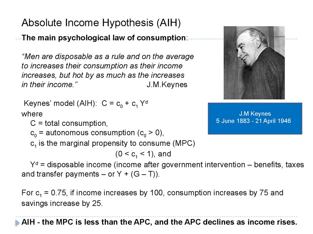
Absolute Income Hypothesis (AIH)
The main psychological law of consumption:
“Men are disposable as a rule and on the average
to increases their consumption as their income
increases, but hot by as much as the increases
in their income.”
J.M.Keynes
Keynes’ model (AIH): C = c0 + c1 Yd
J.M Keynes
where
5 June 1883 - 21 April 1946
C = total consumption,
c0 = autonomous consumption (c0 > 0),
c1 is the marginal propensity to consume (MPC)
(0 < c1 < 1), and
Yd = disposable income (income after government intervention – benefits, taxes
and transfer payments – or Y + (G – T)).
For c1 = 0.75, if income increases by 100, consumption increases by 75 and
photo
savings increase by 25.
AIH - the MPC is less than the APC, and the APC declines as income rises.

4.

How can one test the Absolute Income Hypothesis (AIH)?
photo

5.

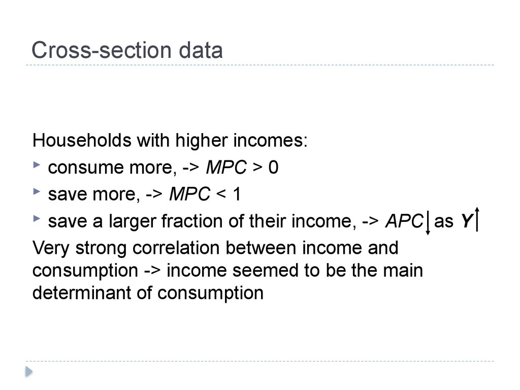
Cross-section data
Households with higher incomes:
consume more, -> MPC > 0
save more, -> MPC < 1
save a larger fraction of their income, -> APC as Y
Very strong correlation between income and
consumption -> income seemed to be the main
determinant of consumption

6.

Kuznets’ critique of AIH
While early empirical work found support for the AIH and the proposition that
the APC falls as income rises, long-run data offered contrary evidence
(Kuznets 1946).
This indicated that the APC out of national disposable income appeared not
to vary with rising income over the relatively long run; in particular, it did
not fall as disposable income rose, as predicted by the linear AIH inclusive
of an intercept.
Rather, the apparent constancy of the APC suggested a long-run
proportional consumption function (C), such that the APC equals the MPC.
photo

7.

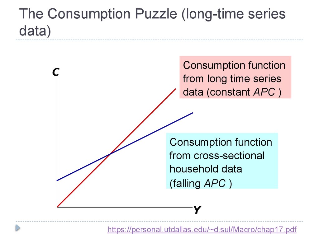
The Consumption Puzzle (long-time series
data)
C
Consumption function
from long time series
data (constant APC )
Consumption function
from cross-sectional
household data
(falling APC )
Y
https://personal.utdallas.edu/~d.sul/Macro/chap17.pdf

8.

Keynes vs. Fisher
Keynes:
Current consumption depends only on current income. Kuznets (1942) has
conducted a long-run consumption function using US’ time series data
from 1897 to 1938. He showed that in the long run, contrary to AIH
assumption APC and MPC are equal and not far from one.
Irving Fisher (1930):
Consumer is forward-looking and chooses consumption for the present
and future to maximize lifetime satisfaction.
Current consumption depends only on the present value of lifetime
income. The timing of income is irrelevant because the consumer can
borrow or lend between periods.
If consumer knows that her future income will increase, she can spread
the extra consumption over both periods by borrowing in the current
period.
However, if consumer faces borrowing constraints (‘liquidity constraints’),
then she may not be able to increase current consumption ...and her
consumption may behave as in the Keynesian theory even though she is
rational & forward-looking. https://personal.utdallas.edu/~d.sul/Macro/chap17.pdf

9.

Permanent income (PIH) & Life-cycle (LCH) hypotheses
as a critical response to Absolute Income Hypothesis (AIH)
Keynes’ model (AIH) failed to explain
consumers’
behaviour accurately:
• econometric concerns including the problem of omitted
variables and autocorrelation;
• Keynes’ predictions about after-war consumption did not
come true.
I. Fisher (1930) – consumer is forward-looking and chooses
consumption for the present and future to maximize lifetime
satisfaction.
Milton Friedman
Milton Friedman
(1912-2006)
M. Friedman and F. Modigliani - theories of PIH and LCH,
both appeared in 1957.
They proposed that current income is not the major factor
influencing consumption/saving decision. Rather, it is the
person’s total life-time income – permanent income, as
Friedman puts it.
Higher School of Economics , Moscow, 2011
photo
Franco Modigliani
(1918-2003)

10.

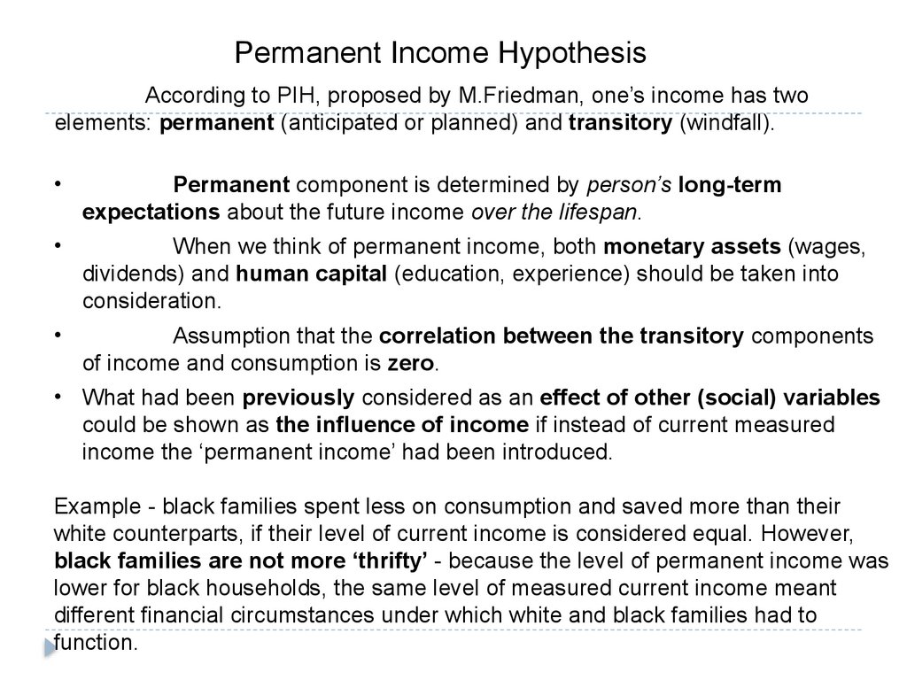
Permanent Income Hypothesis
According to PIH, proposed by M.Friedman, one’s income has two
elements: permanent (anticipated or planned) and transitory (windfall).
Permanent component is determined by person’s long-term
expectations about the future income over the lifespan.
When we think of permanent income, both monetary assets (wages,
dividends) and human capital (education, experience) should be taken into
consideration.
Assumption that the correlation between the transitory components
of income and consumption is zero.
• What had been previously considered as an effect of other (social) variables
could be shown as the influence of income if instead of current measured
income the ‘permanent income’ had been introduced.
Example - black families spent less on consumption and saved more than their
white counterparts, if their level of current income is considered equal. However,
black families are not more ‘thrifty’ - because the level of permanent income was
photo
lower for black households, the same level of measured current income meant
different financial circumstances under which white and black families had to
function.

11.

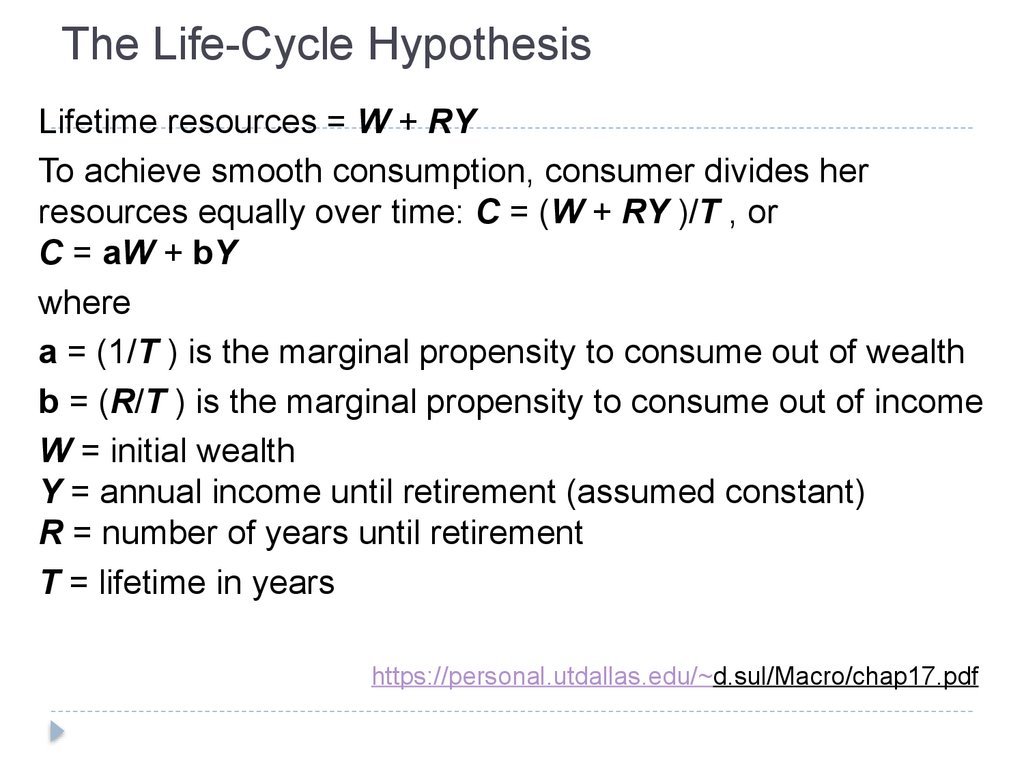
The Life-Cycle Hypothesis
Lifetime resources = W + RY
To achieve smooth consumption, consumer divides her
resources equally over time: C = (W + RY )/T , or
C = aW + bY
where
a = (1/T ) is the marginal propensity to consume out of wealth
b = (R/T ) is the marginal propensity to consume out of income
W = initial wealth
Y = annual income until retirement (assumed constant)
R = number of years until retirement
T = lifetime in years
https://personal.utdallas.edu/~d.sul/Macro/chap17.pdf

12.

Life-Cycle Hypothesis
photo

13.

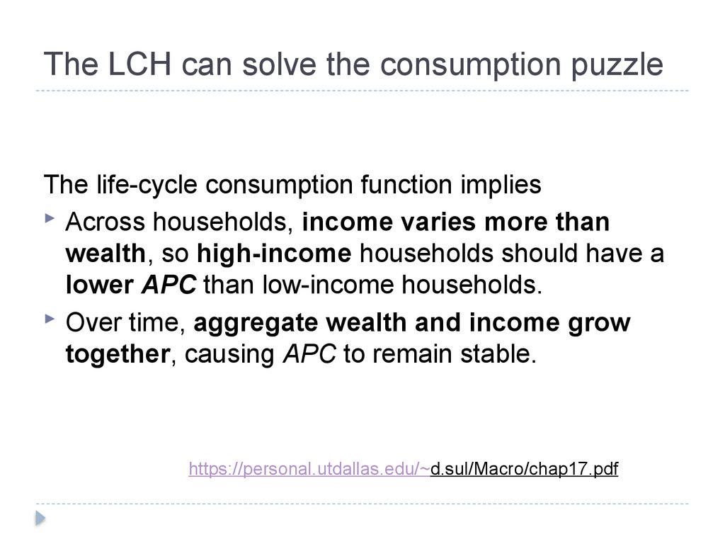
The LCH can solve the consumption puzzle
The life-cycle consumption function implies
Across households, income varies more than
wealth, so high-income households should have a
lower APC than low-income households.
Over time, aggregate wealth and income grow
together, causing APC to remain stable.
https://personal.utdallas.edu/~d.sul/Macro/chap17.pdf

14.

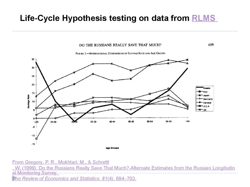
Life-Cycle Hypothesis testing on data from RLMS
photo
From Gregory, P. R., Mokhtari, M., & Schrettl
, W. (1999). Do the Russians Really Save That Much?-Alternate Estimates from the Russian Longitudin
al Monitoring Survey.
The Review of Economics and Statistics, 81(4), 694–703.

15.

Income uncertainty - the main challenge to the
neoclassical consumption and savings models (PIH & LCH)
Why income uncertainty is a big problem?
In PI-LC framework consumption increases with current
income only if that increase is a permanent one
In case of uncertainty individuals can not estimate the
permanent (life-cycle) level of consumption and as a result
are unable to smooth out the fluctuations of income
So, one needs to introduce assumptions about the nature of
uncertainty and preferences, otherwise it is not possible to
obtain a closed form solution for consumption.
Excess sensitivity of consumption to income: consumption
responds too much to predictable changes in income.
The best candidate explanation is the existence of borrowing
(liquidity) constraints.

16.

Consumer response to the Reagan tax cuts - Paper by Nic
holas S.
Souleles
, Journal of Public Economics 85 (2002), pp.99-120
Research question
Reagan tax cut – tax reform. While its second and third stage the reform
was announced in advance.
Phases of Reagan tax cut
1. 5% decrease – October 1981;
10% decrease - July 1982;
3. 10% deacrease – July 1983
the PIH model - consumers should respond to news about their future tax
liability, not to previously expected actual changes in withholding cash
flows.
However, as Souleles noticed, consumption is found to be excessively
sensitive to the tax cuts, counter to the model. Liquidity constraints and
other standard explanations do not appear to explain this excess
sensitivity.
2.

17.

More research on the excess sensitivity of
consumption to income
Wilcox (1989) found that social security recipients
respond not to the announcement of increases in their
benefits, but only later on actually receiving the
increases.
Poterba (1988) concluded that consumption did not
react to news of policy changes, counter to the LC/PI
model.
Fisher et al. (2020) the MPC is lower at higher wealth
quintiles, indicating that low wealth households cannot
smooth consumption as much as other households.
This implies that increasing wealth inequality likely
reduces aggregate consumption, which, in turn, could
limit economic growth

18.

Borrowing (liquidity) constraints
It has now become customary to interpret evidence of 'excess
sensitivity' of consumption growth to labour income as an indication
of 'liquidity constraints', by which it is usually meant the presence of
some imperfection in financial markets that prevents people from
borrowing.
Deaton (1991) estimated the effect of liquidity constraints on the
level of consumption. His conclusion was that the behaviour induced
by the presence of liquidity constraints is similar to that associated
with a precautionary motive for saving. As in the precautionary
motive for saving, people will accumulate a buffer stock to avoid
the possibility of needing a loan that they cannot obtain.
Furthermore, the liquidity constraint will be binding only occasionally
as during most periods, individuals avoid, by their optimal behaviour,
to find themselves constrained.

19.

Buffer-stock saving model
When consumers are both impatient and prudent there will be
a target level of wealth (`cash' for short) such that if actual
cash exceeds the target, the consumer will spend freely
and cash will fall, while if actual cash is below the target the
consumer will save and cash will rise.
Gourinchas and Parker (2002) estimate the model and
conclude that the buffer-stock saving phase of life lasts from
age 25 until around age 40-45.
Carroll (1992) - it can be optimal for average household
spending patterns to mirror average household income
profiles over much of the life cycle.

20.

Bequest motives
One of the implications of the simplest version of the life cycle
model is that wealth is decumulated in the last part of the life
cycle.
While the rate at which wealth is decumulated depends on the
parameters of the model and in particular about beliefs about
longevity, the result that wealth should decline seems to be
robust.
The evidence on this point is mixed, in that several studies do not
find strong evidence of decumulation of wealth by the elderly.

21.

Measuring cohort effects
As the data sets are not panels, to estimate age profiles, researchers
forced to use grouping techniques. These techniques were first used
within life cycle models by Browning, Deaton and Irish (1985).
Rather than following the same individual over time, one can follow tile
average behaviour of a group of individuals as they age. Groups can
be defined in different ways, as long as the membership of the group
is constant over time.
To compute the life cycle profile of a given variable, say log
consumption, one splits the households interviewed in each
individual cross section in groups defined on the basis of the
household head's year of birth.
Their big advantage is that they allow to study the dynamic behaviour
of the variables of interest even in the absence of panel data.
Indeed, in many respects, their use might be superior to that of panel
data! For example, time series of cross sections are probably
less affected by non-random attrition than panel data.

22.

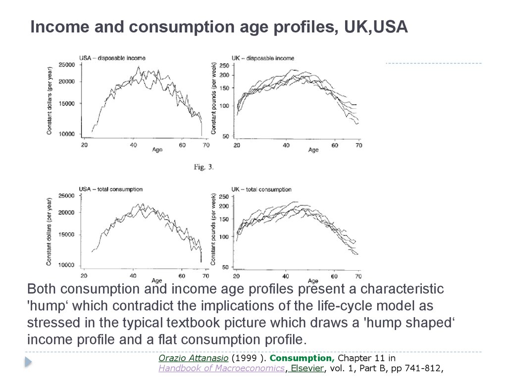
Income and consumption age profiles, UK,USA
Both consumption and income age profiles present a characteristic
'hump‘ which contradict the implications of the life-cycle model as
stressed in the typical textbook picture which draws a 'hump shaped‘
income profile and a flat consumption profile.
Orazio Attanasio (1999 ). Consumption, Chapter 11 in
Handbook of Macroeconomics, Elsevier, vol. 1, Part B, pp 741-812,

23.

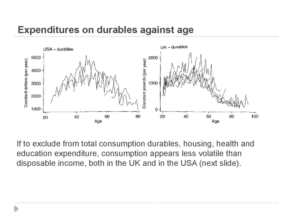
Expenditures on durables against age
If to exclude from total consumption durables, housing, health and
education expenditure, consumption appears less volatile than
disposable income, both in the UK and in the USA (next slide).

24.

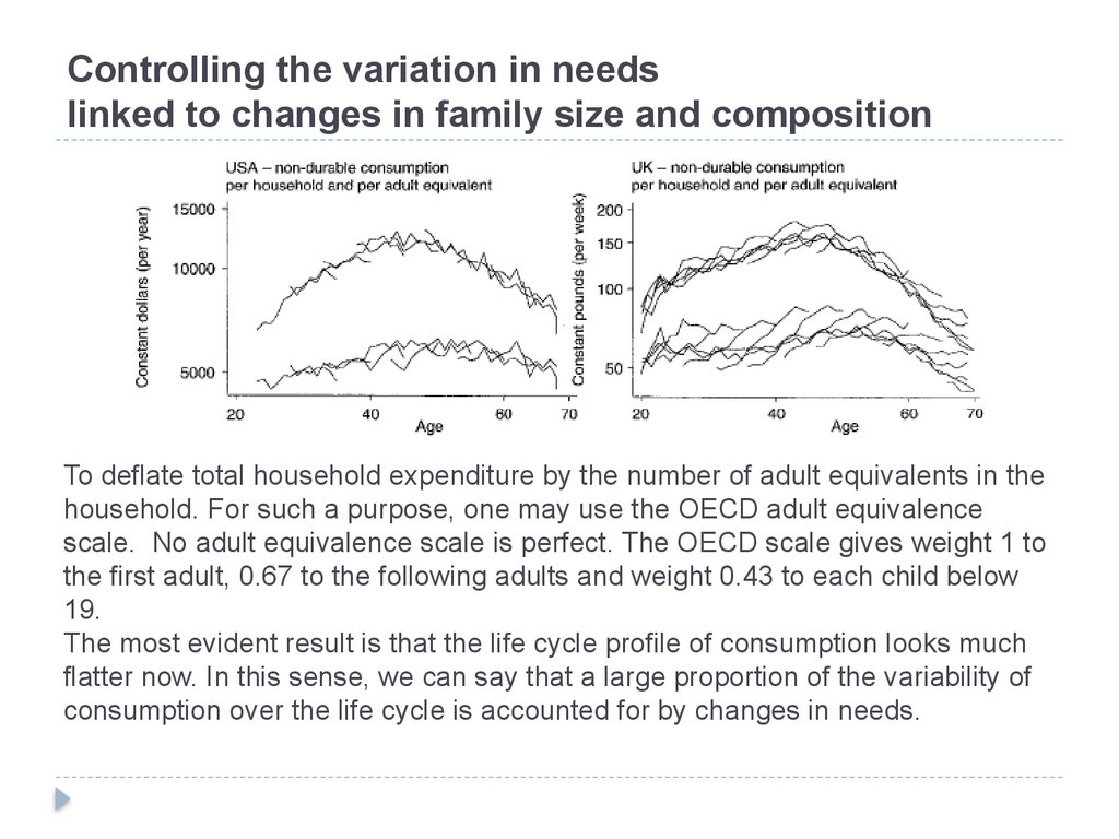
Controlling the variation in needs
linked to changes in family size and composition
To deflate total household expenditure by the number of adult equivalents in the
household. For such a purpose, one may use the OECD adult equivalence
scale. No adult equivalence scale is perfect. The OECD scale gives weight 1 to
the first adult, 0.67 to the following adults and weight 0.43 to each child below
19.
The most evident result is that the life cycle profile of consumption looks much
flatter now. In this sense, we can say that a large proportion of the variability of
consumption over the life cycle is accounted for by changes in needs.