CS240A: Conjugate Gradients and the Model Problem

1.

CS240A: Conjugate Gradients
and the Model Problem

2.

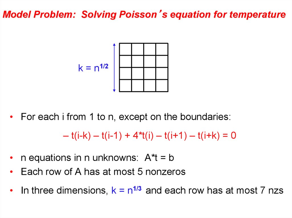
Model Problem: Solving Poisson’s equation for temperature
k = n1/2
• For each i from 1 to n, except on the boundaries:
– t(i-k) – t(i-1) + 4*t(i) – t(i+1) – t(i+k) = 0
• n equations in n unknowns: A*t = b
• Each row of A has at most 5 nonzeros
• In three dimensions, k = n1/3 and each row has at most 7 nzs

3.

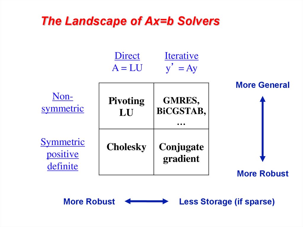
The Landscape of Ax=b Solvers
Direct
A = LU
Iterative
y’ = Ay
More General
Nonsymmetric
Pivoting
LU
GMRES,
BiCGSTAB,
…
Symmetric
positive
definite
Cholesky
Conjugate
gradient
More Robust
More Robust
Less Storage (if sparse)

4.

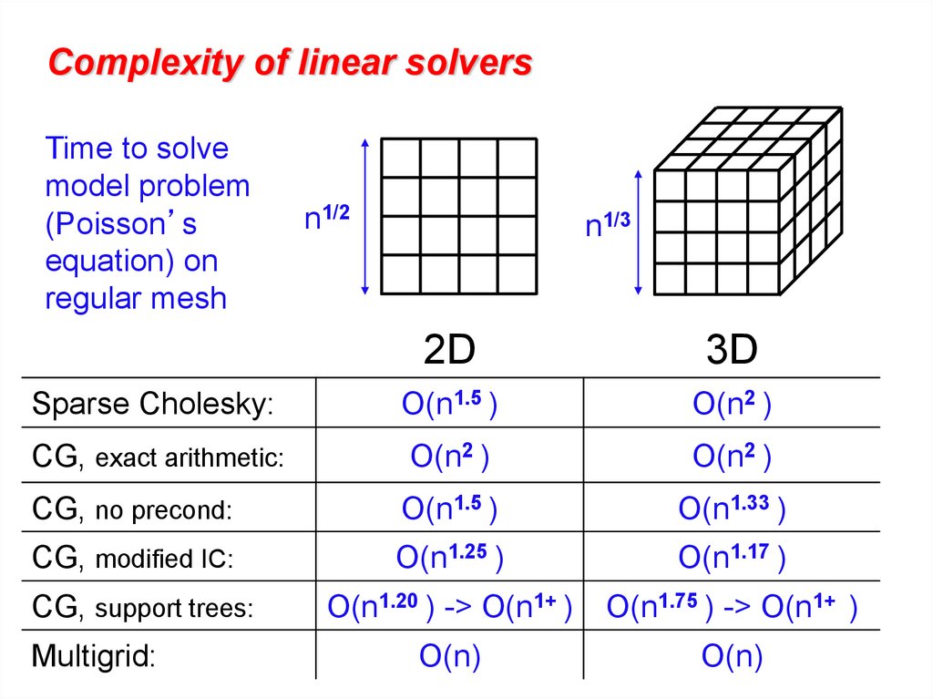
Complexity of linear solvers
Time to solve
model problem
(Poisson’s
equation) on
regular mesh
n1/2
n1/3
2D
3D
Sparse Cholesky:
O(n1.5 )
O(n2 )
CG, exact arithmetic:
O(n2 )
O(n2 )
CG, no precond:
O(n1.5 )
O(n1.33 )
CG, modified IC:
O(n1.25 )
O(n1.17 )
CG, support trees:
O(n1.20 ) -> O(n1+ )
O(n1.75 ) -> O(n1+ )
O(n)
O(n)
Multigrid:

5.

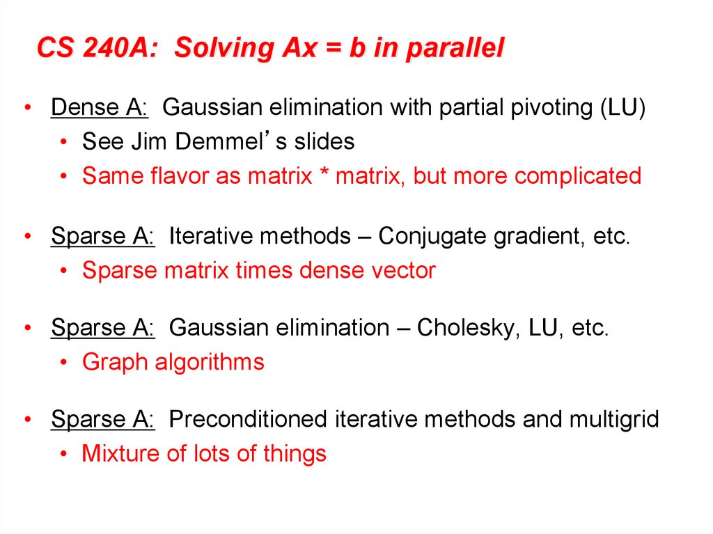
CS 240A: Solving Ax = b in parallel
• Dense A: Gaussian elimination with partial pivoting (LU)
• See Jim Demmel’s slides
• Same flavor as matrix * matrix, but more complicated
• Sparse A: Iterative methods – Conjugate gradient, etc.
• Sparse matrix times dense vector
• Sparse A: Gaussian elimination – Cholesky, LU, etc.
• Graph algorithms
• Sparse A: Preconditioned iterative methods and multigrid
• Mixture of lots of things

6.

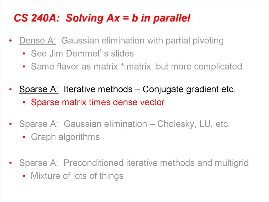
CS 240A: Solving Ax = b in parallel
• Dense A: Gaussian elimination with partial pivoting
• See Jim Demmel’s slides
• Same flavor as matrix * matrix, but more complicated
• Sparse A: Iterative methods – Conjugate gradient etc.
• Sparse matrix times dense vector
• Sparse A: Gaussian elimination – Cholesky, LU, etc.
• Graph algorithms
• Sparse A: Preconditioned iterative methods and multigrid
• Mixture of lots of things

7.

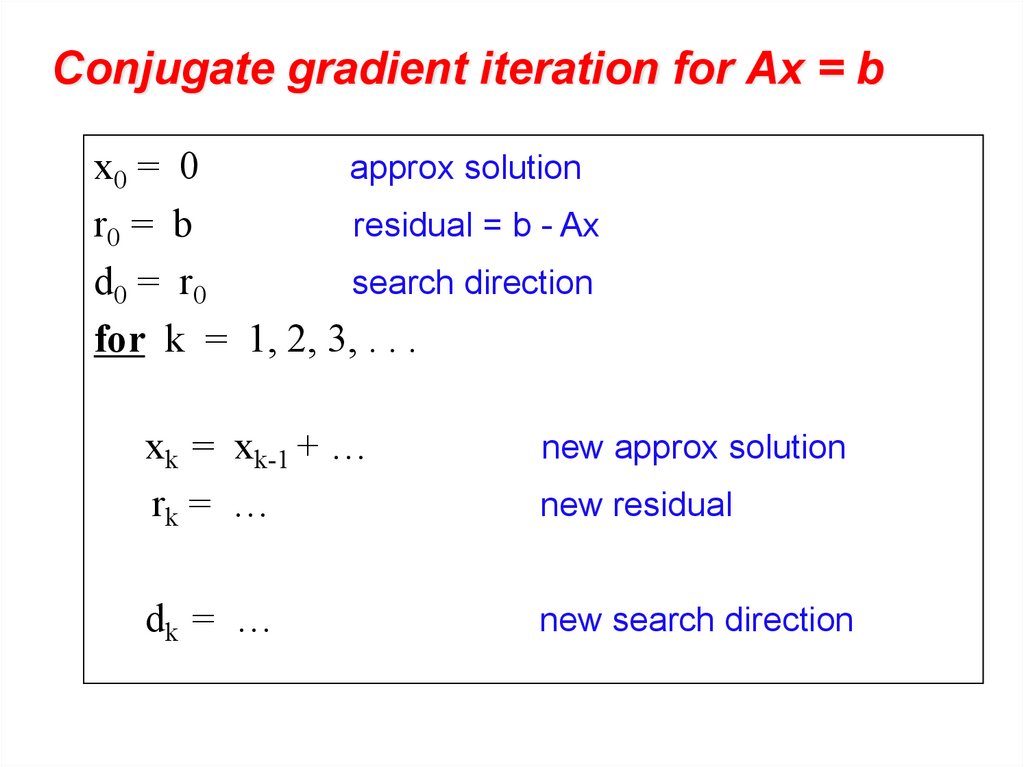
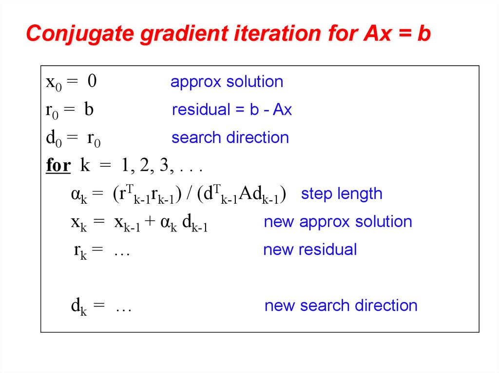
Conjugate gradient iteration for Ax = b
x0 = 0
approx solution
r0 = b
residual = b - Ax
d0 = r0
search direction
for k = 1, 2, 3, . . .
xk = xk-1 + …
rk = …
new residual
dk = …
new search direction
new approx solution

8.

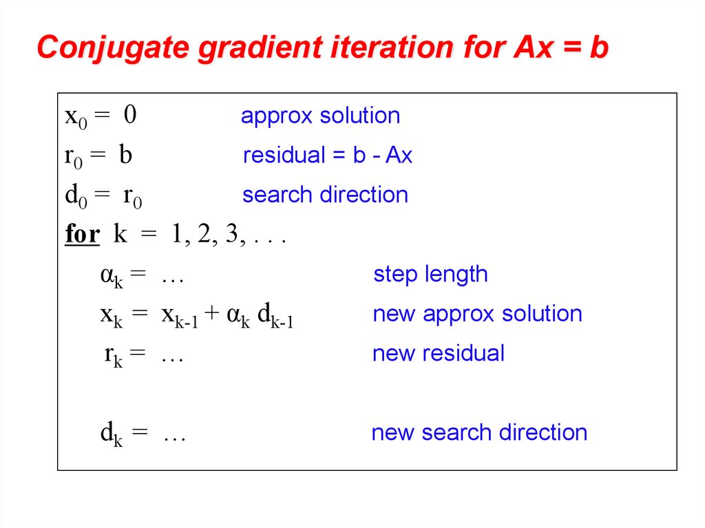
Conjugate gradient iteration for Ax = b
x0 = 0
approx solution
r0 = b
residual = b - Ax
d0 = r0
search direction
for k = 1, 2, 3, . . .
αk = …
step length
xk = xk-1 + αk dk-1
new approx solution
rk = …
new residual
dk = …
new search direction

9.

Conjugate gradient iteration for Ax = b
x0 = 0
approx solution
r0 = b
residual = b - Ax
d0 = r0
search direction
for k = 1, 2, 3, . . .
αk = (rTk-1rk-1) / (dTk-1Adk-1) step length
xk = xk-1 + αk dk-1
new approx solution
rk = …
new residual
dk = …
new search direction

10.

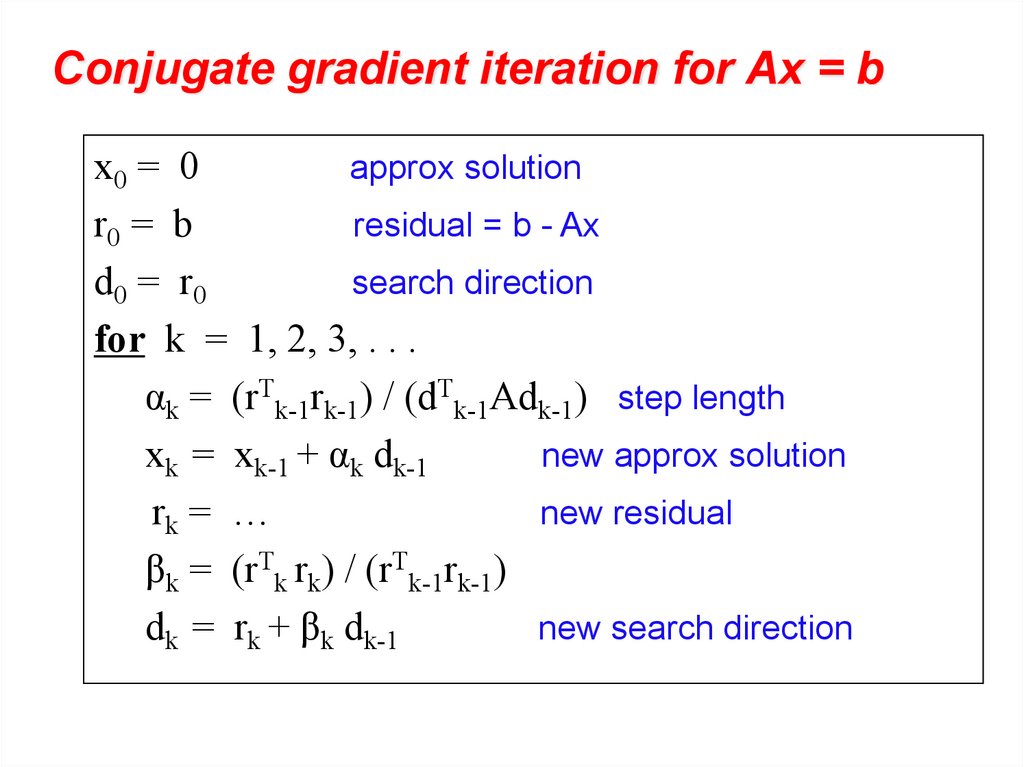
Conjugate gradient iteration for Ax = b
x0 = 0
approx solution
r0 = b
residual = b - Ax
d0 = r0
search direction
for k = 1, 2, 3, . . .
αk = (rTk-1rk-1) / (dTk-1Adk-1) step length
xk = xk-1 + αk dk-1
new approx solution
rk = …
new residual
βk = (rTk rk) / (rTk-1rk-1)
dk = rk + βk dk-1
new search direction

11.

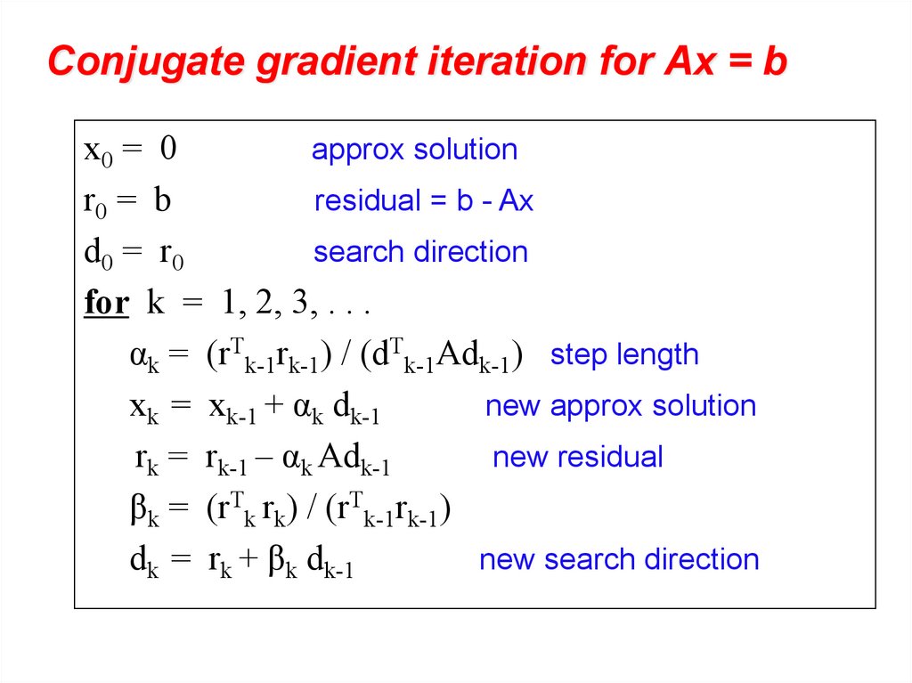
Conjugate gradient iteration for Ax = b
x0 = 0
approx solution
r0 = b
residual = b - Ax
d0 = r0
search direction
for k = 1, 2, 3, . . .
αk = (rTk-1rk-1) / (dTk-1Adk-1) step length
xk = xk-1 + αk dk-1
new approx solution
rk = rk-1 – αk Adk-1
new residual
βk = (rTk rk) / (rTk-1rk-1)
dk = rk + βk dk-1
new search direction

12.

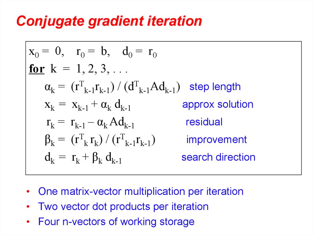
Conjugate gradient iteration
x0 = 0, r0 = b, d0 = r0
for k = 1, 2, 3, . . .
αk = (rTk-1rk-1) / (dTk-1Adk-1) step length
xk = xk-1 + αk dk-1
approx solution
rk = rk-1 – αk Adk-1
residual
βk = (rTk rk) / (rTk-1rk-1)
improvement
dk = rk + βk dk-1
search direction
• One matrix-vector multiplication per iteration
• Two vector dot products per iteration
• Four n-vectors of working storage

13.

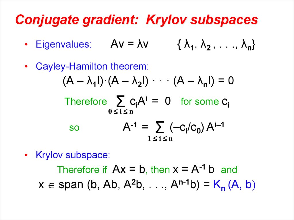
Conjugate gradient: Krylov subspaces
• Eigenvalues:
Av = λv
{ λ1, λ2 , . . ., λn}
• Cayley-Hamilton theorem:
(A – λ1I)·(A – λ2I) · · · (A – λnI) = 0
Therefore
so
ciAi = 0 for some ci
Σ
0 i n
A-1 = Σ (–ci/c0) Ai–1
1 i n
• Krylov subspace:
Therefore if Ax = b, then x = A-1 b and
x span (b, Ab, A2b, . . ., An-1b) = Kn (A, b)

14.

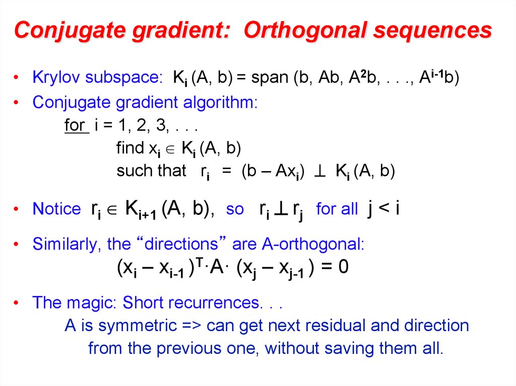
Conjugate gradient: Orthogonal sequences
• Krylov subspace: Ki (A, b) = span (b, Ab, A2b, . . ., Ai-1b)
• Conjugate gradient algorithm:
for i = 1, 2, 3, . . .
find xi Ki (A, b)
such that ri = (b – Axi) Ki (A, b)
• Notice ri Ki+1 (A, b), so ri rj for all j < i
• Similarly, the “directions” are A-orthogonal:
(xi – xi-1 )T·A· (xj – xj-1 ) = 0
• The magic: Short recurrences. . .
A is symmetric => can get next residual and direction
from the previous one, without saving them all.

15.

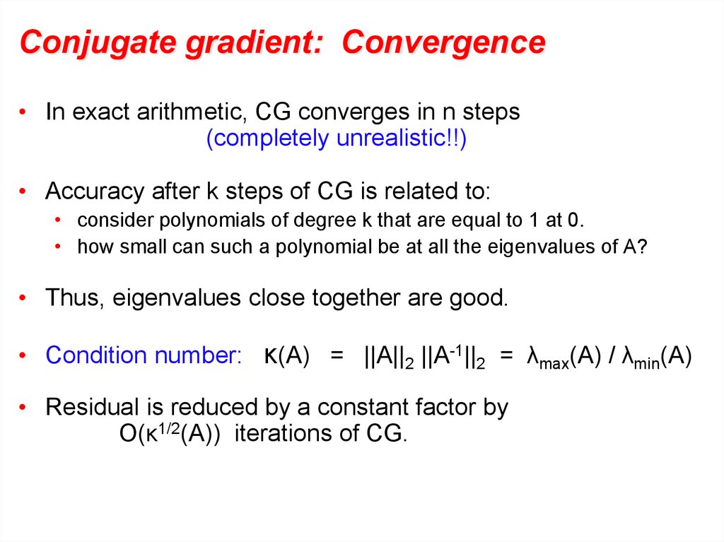
Conjugate gradient: Convergence
• In exact arithmetic, CG converges in n steps
(completely unrealistic!!)
• Accuracy after k steps of CG is related to:
• consider polynomials of degree k that are equal to 1 at 0.
• how small can such a polynomial be at all the eigenvalues of A?
• Thus, eigenvalues close together are good.
• Condition number: κ(A) = ||A||2 ||A-1||2 = λmax(A) / λmin(A)
• Residual is reduced by a constant factor by
O(κ1/2(A)) iterations of CG.

16.

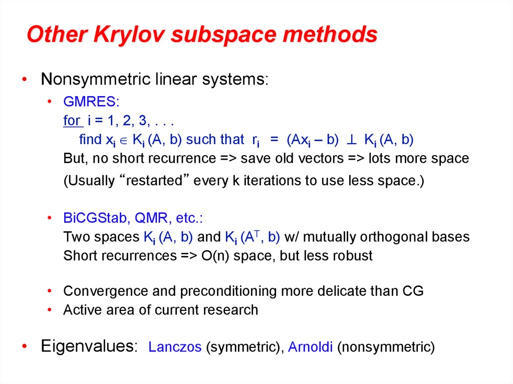
Other Krylov subspace methods
• Nonsymmetric linear systems:
• GMRES:
for i = 1, 2, 3, . . .
find xi Ki (A, b) such that ri = (Axi – b) Ki (A, b)
But, no short recurrence => save old vectors => lots more space
(Usually “restarted” every k iterations to use less space.)
• BiCGStab, QMR, etc.:
Two spaces Ki (A, b) and Ki (AT, b) w/ mutually orthogonal bases
Short recurrences => O(n) space, but less robust
• Convergence and preconditioning more delicate than CG
• Active area of current research
• Eigenvalues: Lanczos (symmetric), Arnoldi (nonsymmetric)

17.

Conjugate gradient iteration
x0 = 0, r0 = b, d0 = r0
for k = 1, 2, 3, . . .
αk = (rTk-1rk-1) / (dTk-1Adk-1) step length
xk = xk-1 + αk dk-1
approx solution
rk = rk-1 – αk Adk-1
residual
βk = (rTk rk) / (rTk-1rk-1)
improvement
dk = rk + βk dk-1
search direction
• One matrix-vector multiplication per iteration
• Two vector dot products per iteration
• Four n-vectors of working storage

18.

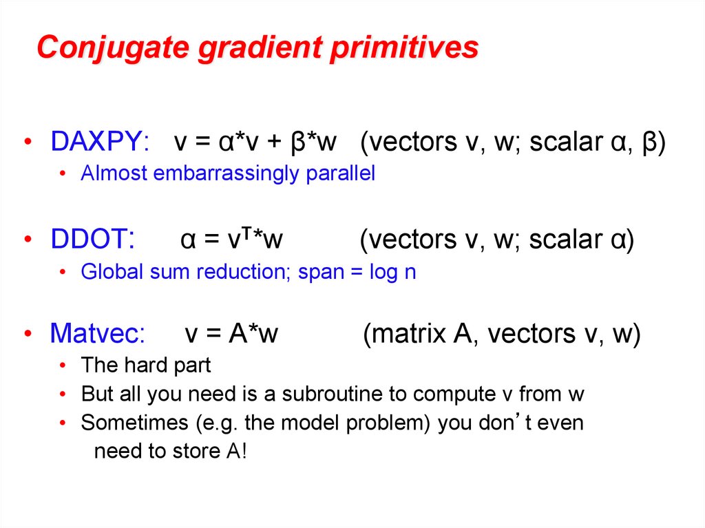
Conjugate gradient primitives
• DAXPY: v = α*v + β*w (vectors v, w; scalar α, β)
• Almost embarrassingly parallel
• DDOT:
α = vT*w
(vectors v, w; scalar α)
• Global sum reduction; span = log n
• Matvec:
v = A*w
(matrix A, vectors v, w)
• The hard part
• But all you need is a subroutine to compute v from w
• Sometimes (e.g. the model problem) you don’t even
need to store A!

19.

Model Problem: Solving Poisson’s equation for temperature
k = n1/2
• For each i from 1 to n, except on the boundaries:
– t(i-k) – t(i-1) + 4*t(i) – t(i+1) – t(i+k) = 0
• n equations in n unknowns: A*t = b
• Each row of A has at most 5 nonzeros
• In three dimensions, k = n1/3 and each row has at most 7 nzs

20.

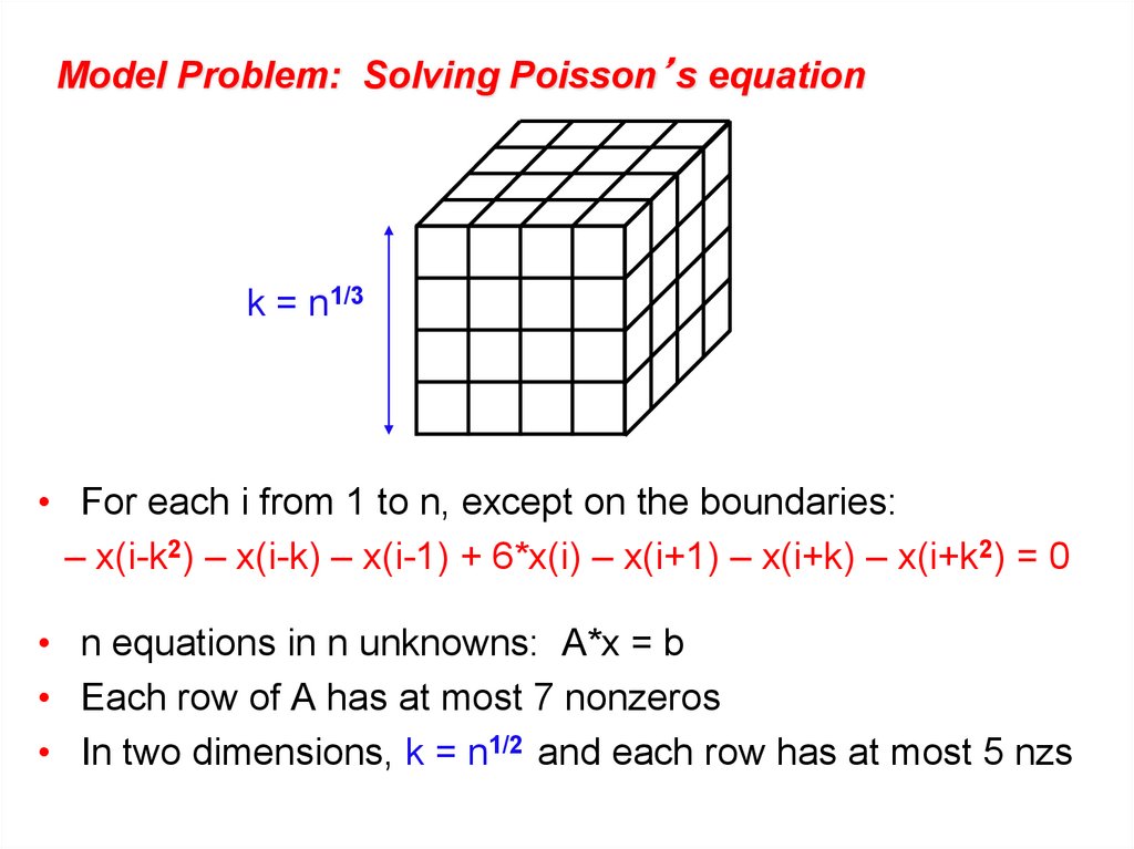
Model Problem: Solving Poisson’s equation
k = n1/3
• For each i from 1 to n, except on the boundaries:
– x(i-k2) – x(i-k) – x(i-1) + 6*x(i) – x(i+1) – x(i+k) – x(i+k2) = 0
• n equations in n unknowns: A*x = b
• Each row of A has at most 7 nonzeros
• In two dimensions, k = n1/2 and each row has at most 5 nzs

21.

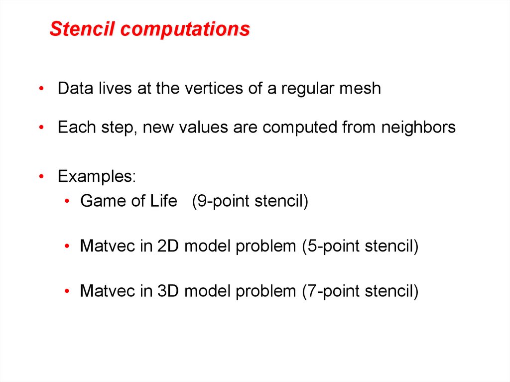
Stencil computations
• Data lives at the vertices of a regular mesh
• Each step, new values are computed from neighbors
• Examples:
• Game of Life (9-point stencil)
• Matvec in 2D model problem (5-point stencil)
• Matvec in 3D model problem (7-point stencil)

22.

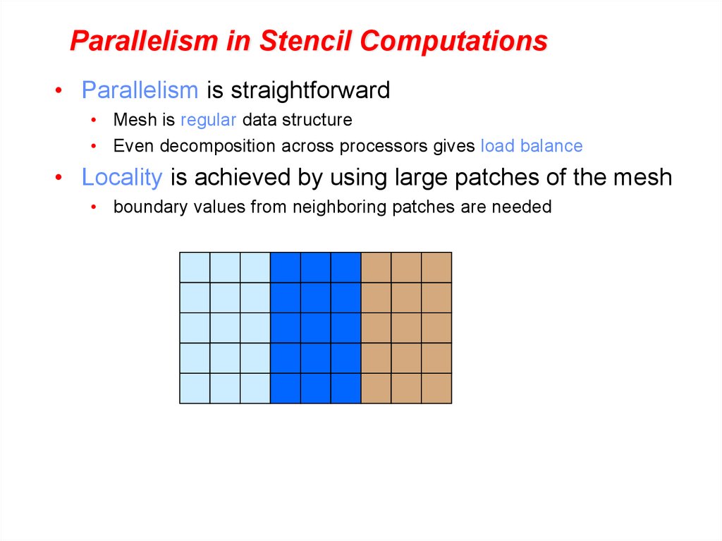
Parallelism in Stencil Computations
• Parallelism is straightforward
• Mesh is regular data structure
• Even decomposition across processors gives load balance
• Locality is achieved by using large patches of the mesh
• boundary values from neighboring patches are needed

23.

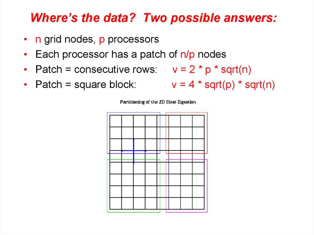
Where’s the data? Two possible answers:
n grid nodes, p processors
Each processor has a patch of n/p nodes
Patch = consecutive rows: v = 2 * p * sqrt(n)
Patch = square block:
v = 4 * sqrt(p) * sqrt(n)

24.

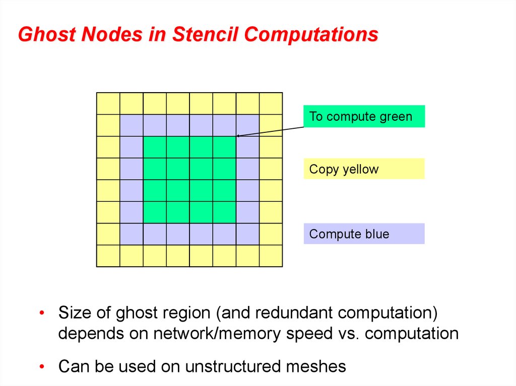
Ghost Nodes in Stencil Computations
To compute green
Copy yellow
Compute blue
• Size of ghost region (and redundant computation)
depends on network/memory speed vs. computation
• Can be used on unstructured meshes