Introduction to Neural Networks

1.

Introduction to Neural Networks.

2.

2
Bibliography
1. Madan M. Gupta, Liang Jin, Noriyasu Homma. Static and
Dynamic Neural Networks: From Fundamentals to Advanced
Theory. John Wiley & Sons, Hoboken, New Jersey. 2003.
2. The handbook of brain theory and neural networks / Michael
A. Arbib, editor - 2nd ed. THE MIT PRESS. Cambridge,
Massachusetts. London, England. 2003.
3. Nikhil Buduma and Nicholas Lacascio. Fundamentals of Deep
Learning. Designing Next-Generation Machine Intelligence
Algorithms. O’Reilly Media, US. 2017.
4. Pshikhopov, V.Kh. (Ed.), Beloglazov D., Finaev V., Guzik V.,
Kosenko E., Krukhmalev V., Medvedev M., Pereverzev V.,
Pyavchenko A., Saprykin R., Shapovalov I., Soloviev V.
(2017). Path Planning for Vehicles Operating in Uncertain 2D
Environments, Elsevier, Butterworth-Heinemann, 312p.

3.

3
Contents
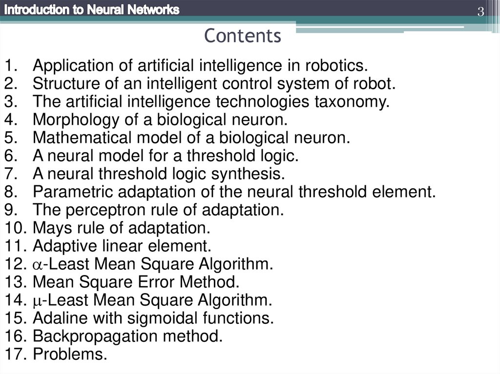
1. Application of artificial intelligence in robotics.
2. Structure of an intelligent control system of robot.
3. The artificial intelligence technologies taxonomy.
4. Morphology of a biological neuron.
5. Mathematical model of a biological neuron.
6. A neural model for a threshold logic.
7. A neural threshold logic synthesis.
8. Parametric adaptation of the neural threshold element.
9. The perceptron rule of adaptation.
10. Mays rule of adaptation.
11. Adaptive linear element.
12. -Least Mean Square Algorithm.
13. Mean Square Error Method.
14. -Least Mean Square Algorithm.
15. Adaline with sigmoidal functions.
16. Backpropagation method.
17. Problems.

4.

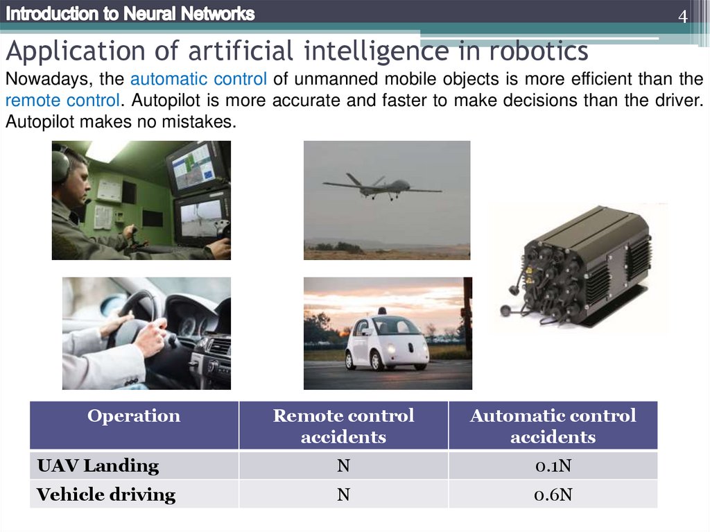
4
Application of artificial intelligence in robotics
Nowadays, the automatic control of unmanned mobile objects is more efficient than the
remote control. Autopilot is more accurate and faster to make decisions than the driver.
Autopilot makes no mistakes.
Operation
Remote control
accidents
Automatic control
accidents
UAV Landing
N
0.1N
Vehicle driving
N
0.6N

5.

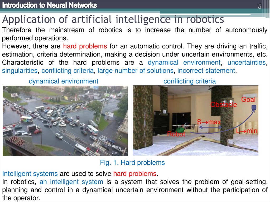
5
Application of artificial intelligence in robotics
Therefore the mainstream of robotics is to increase the number of autonomously
performed operations.
However, there are hard problems for an automatic control. They are driving an traffic,
estimation, criteria determination, making a decision under uncertain environments, etc.
Characteristic of the hard problems are a dynamical environment, uncertainties,
singularities, conflicting criteria, large number of solutions, incorrect statement.
dynamical environment
conflicting criteria
Obstacle
Goal
S max
Robot
L min
Fig. 1. Hard problems
Intelligent systems are used to solve hard problems.
In robotics, an intelligent system is a system that solves the problem of goal-setting,
planning and control in a dynamical uncertain environment without the participation of
the operator.

6.

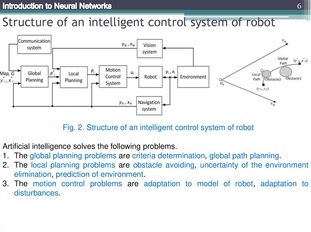
6
Structure of an intelligent control system of robot
Fig. 2. Structure of an intelligent control system of robot
Artificial intelligence solves the following problems.
1. The global planning problems are criteria determination, global path planning.
2. The local planning problems are obstacle avoiding, uncertainty of the environment
elimination, prediction of environment.
3. The motion control problems are adaptation to model of robot, adaptation to
disturbances.

7.

7
The artificial intelligence technologies taxonomy
The artificial intelligence approaches are based on different technologies.
1. An expert knowledge base emulates the experience of the experts in the subject area.
Examples are diagnostic systems in medicine and engineering. Advantage of an expert
knowledge base is unlimited numbers of an expert. Disadvantage is difficulty of the
expert coping. Expert knowledge bases are used as recommendation systems.
2. Fuzzy logic emulates a human cognitive functions (learning, thinking, reasoning, and
adaptation) by uncertain sets. Fuzzy logic uses uncertain notations like “big velocity”,
“low temperature”, etc. The main trait of fuzzy logic is uncertain boundaries between
fuzzy sets. Fuzzy logic is applied for a decision making problem.
3. Evolutionary algorithms emulates the mechanisms of natural selection. The most
known evolutionary algorithm is a genetic algorithm. Evolutionary algorithms are applied
for a global search of the optimal solutions instead of the brute-force searching.
4. Bio-inspired algorithms emulates individual and cooperative behavior of living nature.
Well known bio-inspired algorithms are ant algorithms, pigeon algorithms, and bee
algorithms.
5. Artificial Neural Network is a mathematical model of a human brain. Neural networks
are used as learning systems.

8.

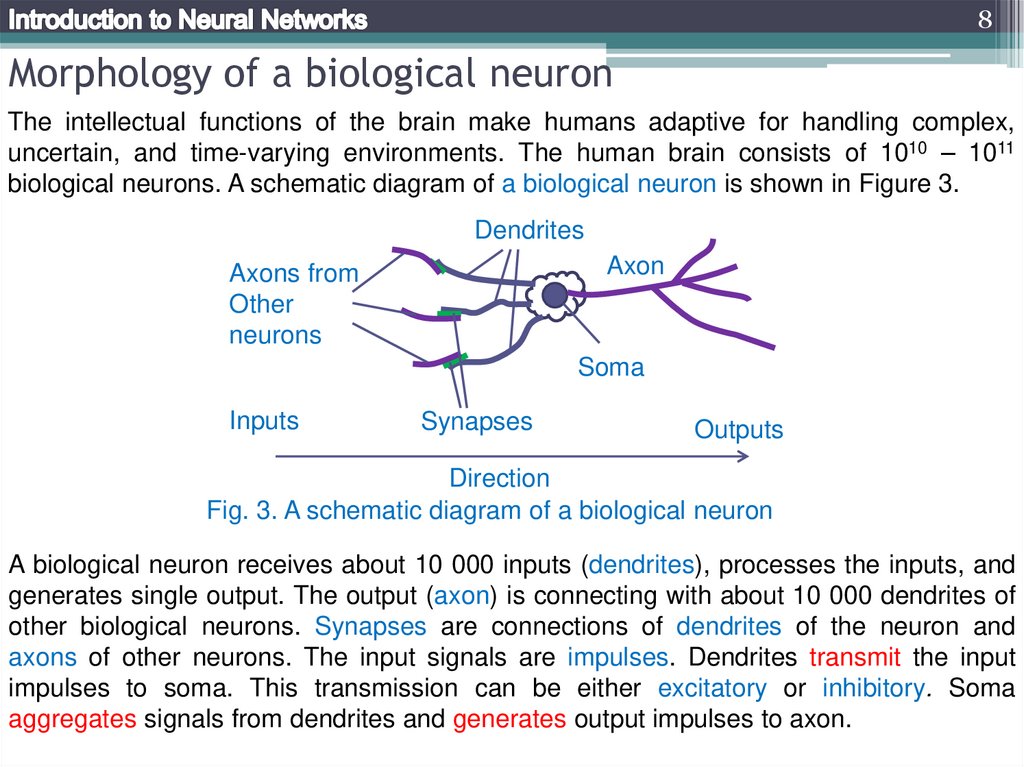
8
Morphology of a biological neuron
The intellectual functions of the brain make humans adaptive for handling complex,
uncertain, and time-varying environments. The human brain consists of 1010 – 1011
biological neurons. A schematic diagram of a biological neuron is shown in Figure 3.
Dendrites
Axon
Axons from
Other
neurons
Soma
Inputs
Synapses
Outputs
Direction
Fig. 3. A schematic diagram of a biological neuron
A biological neuron receives about 10 000 inputs (dendrites), processes the inputs, and
generates single output. The output (axon) is connecting with about 10 000 dendrites of
other biological neurons. Synapses are connections of dendrites of the neuron and
axons of other neurons. The input signals are impulses. Dendrites transmit the input
impulses to soma. This transmission can be either excitatory or inhibitory. Soma
aggregates signals from dendrites and generates output impulses to axon.

9.

9
Mathematical model of a biological neuron
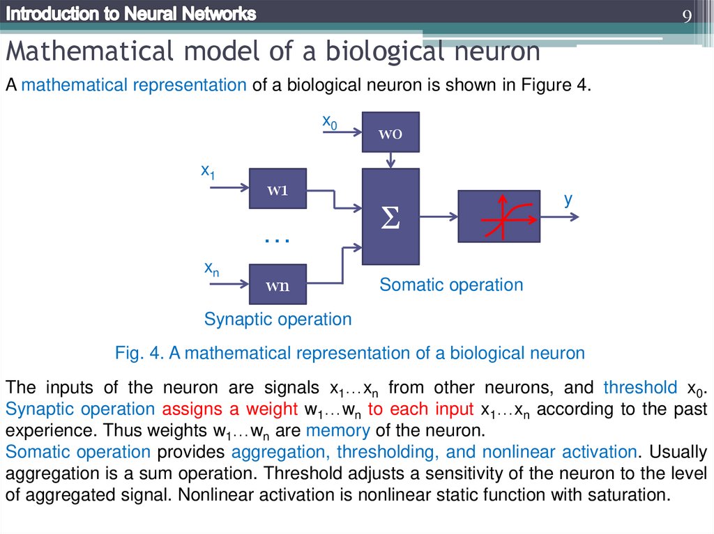
A mathematical representation of a biological neuron is shown in Figure 4.
x0
x1
w1
…
xn
w0
wn
Σ
y
Somatic operation
Synaptic operation
Fig. 4. A mathematical representation of a biological neuron
The inputs of the neuron are signals x1…xn from other neurons, and threshold x0.
Synaptic operation assigns a weight w1…wn to each input x1…xn according to the past
experience. Thus weights w1…wn are memory of the neuron.
Somatic operation provides aggregation, thresholding, and nonlinear activation. Usually
aggregation is a sum operation. Threshold adjusts a sensitivity of the neuron to the level
of aggregated signal. Nonlinear activation is nonlinear static function with saturation.

10.

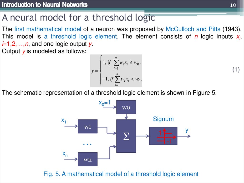
10
A neural model for a threshold logic
The first mathematical model of a neuron was proposed by McCulloch and Pitts (1943).
This model is a threshold logic element. The element consists of n logic inputs xi,
i=1,2,…,n, and one logic output y.
Output y is modeled as follows:
n
1, if wi xi w0 ,
i 1
y
n
1, if w x w .
ii 0
i 1
(1)
The schematic representation of a threshold logic element is shown in Figure 5.
x0=1
x1
Signum
w1
…
xn
w0
Σ
y
1
-1
wn
Fig. 5. A mathematical model of a threshold logic element

11.

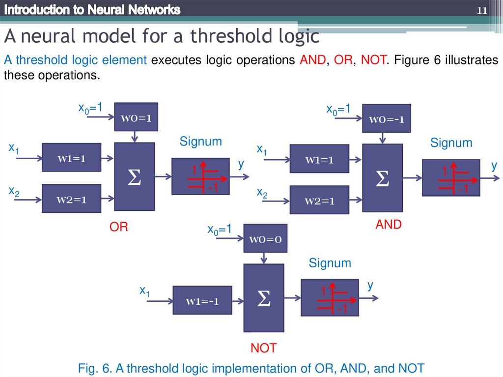
11
A neural model for a threshold logic
A threshold logic element executes logic operations AND, OR, NOT. Figure 6 illustrates
these operations.
x0=1
x1
x2
x0=1
w0=1
Signum
w1=1
Σ
w2=1
OR
x1
y
1
-1
x0=1
x2
w0=-1
Signum
w1=1
Σ
w2=1
AND
w0=0
Signum
x1
w1=-1
Σ
y
1
-1
NOT
Fig. 6. A threshold logic implementation of OR, AND, and NOT
y
1
-1

12.

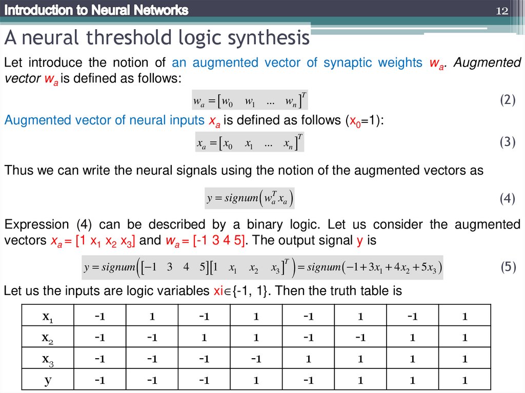
12
A neural threshold logic synthesis
Let introduce the notion of an augmented vector of synaptic weights wa. Augmented
vector wa is defined as follows:
wa w0
w1 ... wn
(2)
T
Augmented vector of neural inputs xa is defined as follows (x0=1):
xa x0
x1 ... xn
(3)
T
Thus we can write the neural signals using the notion of the augmented vectors as
y signum waT xa
(4)
Expression (4) can be described by a binary logic. Let us consider the augmented
vectors xa = [1 x1 x2 x3] and wa = [-1 3 4 5]. The output signal y is
y signum 1 3 4 5 1 x1
x2
x3
T
signum 1 3x 4x 5x
1
2
(5)
3
Let us the inputs are logic variables xi {-1, 1}. Then the truth table is
x1
-1
1
-1
1
-1
1
-1
1
x2
-1
-1
1
1
-1
-1
1
1
x3
-1
-1
-1
-1
1
1
1
1
y
-1
-1
-1
1
-1
1
1
1

13.

13
A neural threshold logic synthesis
From the truth table we obtain
y x1 x2 x3 x2 x3 x2 x3
(6)
Let us consider the following logic function
(7)
y x1 x2 x3
Output y=-1 for both x1x2x3 and not(x1x2x3). Therefore
w1 w2 w3 w0 , and w1 w2 w3 w0
The last inequalities are conflicting. Thus no weights and threshold values can satisfy
them. Function (7) can not be realized by a single threshold element.
A switching function that can be realized by a single threshold element is called a
threshold function. A threshold function is also called a linearly separable function. It
means that hyper plane waTxa divides all values of a threshold function in the next way.
All the true points are on one side of the hyperplane, and the false points are on the
other side of the hyper plane.
x2
y=1
y=-1
y=-1
y=1
x1
x1
y=-1
y=-1
a linearly separable function
y=-1
y=1
a linearly non-separable function (XOR)

14.

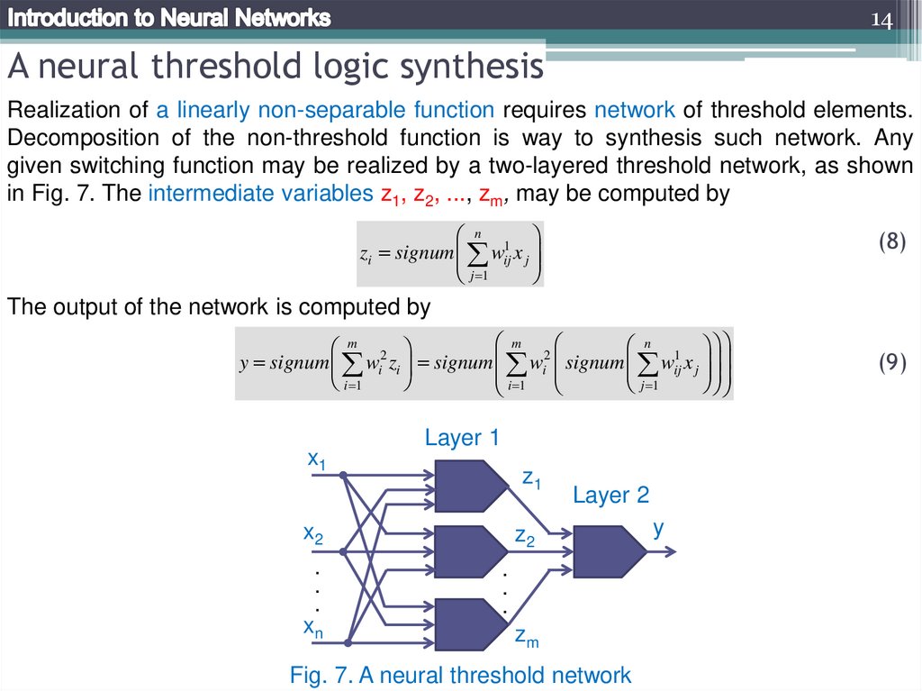
14
A neural threshold logic synthesis
Realization of a linearly non-separable function requires network of threshold elements.
Decomposition of the non-threshold function is way to synthesis such network. Any
given switching function may be realized by a two-layered threshold network, as shown
in Fig. 7. The intermediate variables z1, z2, ..., zm, may be computed by
n 1
zi signum wij x j
j 1
(8)
The output of the network is computed by
m
n 1
m 2
2
y signum wi zi signum wi signum wij x j
j 1
i 1
i 1
x1
Layer 1
z1
x2
.
.
.
xn
Layer 2
z2
.
.
.
zm
Fig. 7. A neural threshold network
y
(9)

15.

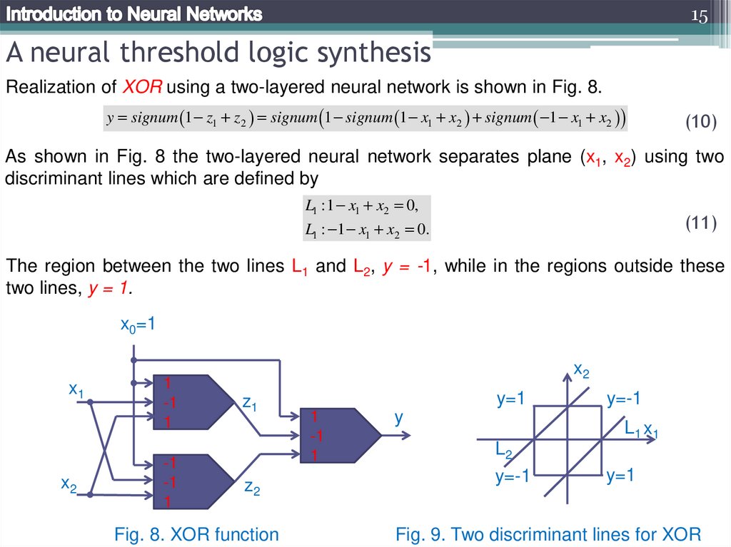
15
A neural threshold logic synthesis
Realization of XOR using a two-layered neural network is shown in Fig. 8.
y signum 1 z1 z2 signum 1 signum 1 x1 x2 signum 1 x1 x2
(10)
As shown in Fig. 8 the two-layered neural network separates plane (x1, x2) using two
discriminant lines which are defined by
L1 :1 x1 x2 0,
(11)
L1 : 1 x1 x2 0.
The region between the two lines L1 and L2, y = -1, while in the regions outside these
two lines, y = 1.
x0=1
x1
x2
1
-1
1
-1
-1
1
x2
z1
z2
Fig. 8. XOR function
y=1
1
-1
1
y
y=-1
L1 x1
L2
y=-1
y=1
Fig. 9. Two discriminant lines for XOR

16.

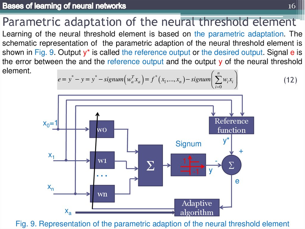
16
Parametric adaptation of the neural threshold element
Learning of the neural threshold element is based on the parametric adaptation. The
schematic representation of the parametric adaption of the neural threshold element is
shown in Fig. 9. Output y* is called the reference output or the desired output. Signal e is
the error between the and the reference output and the output y of the neural threshold
element.
n
*
*
T
*
e y y y signum wa xa f x1 ,..., xn signum wi xi
(12)
i 0
x0=1
Reference
function
y*
+
-
w0
Signum
x1
w1
…
xn
Σ
1
-1
y
e
wn
Adaptive
xa
algorithm
Fig. 9. Representation of the parametric adaption of the neural threshold element

17.

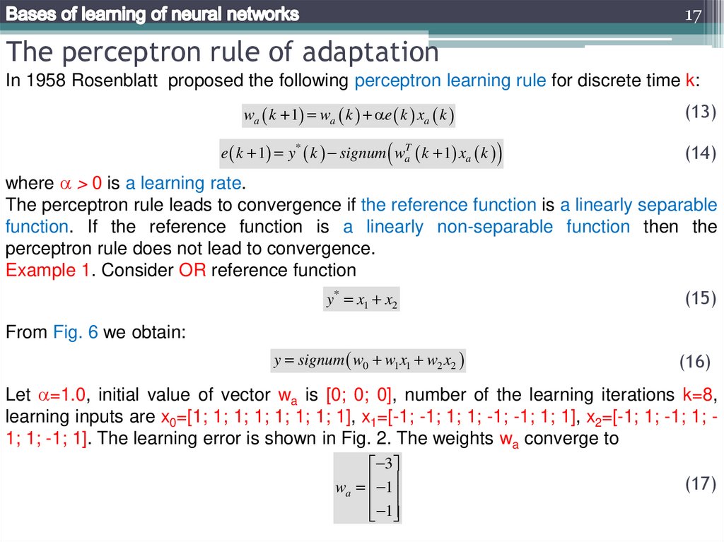
17
The perceptron rule of adaptation
In 1958 Rosenblatt proposed the following perceptron learning rule for discrete time k:
wa k 1 wa k e k xa k
e k 1 y* k signum waT k 1 xa k
(13)
(14)
where > 0 is a learning rate.
The perceptron rule leads to convergence if the reference function is a linearly separable
function. If the reference function is a linearly non-separable function then the
perceptron rule does not lead to convergence.
Example 1. Consider OR reference function
y* x1 x2
(15)
y signum w0 w1 x1 w2 x2
(16)
From Fig. 6 we obtain:
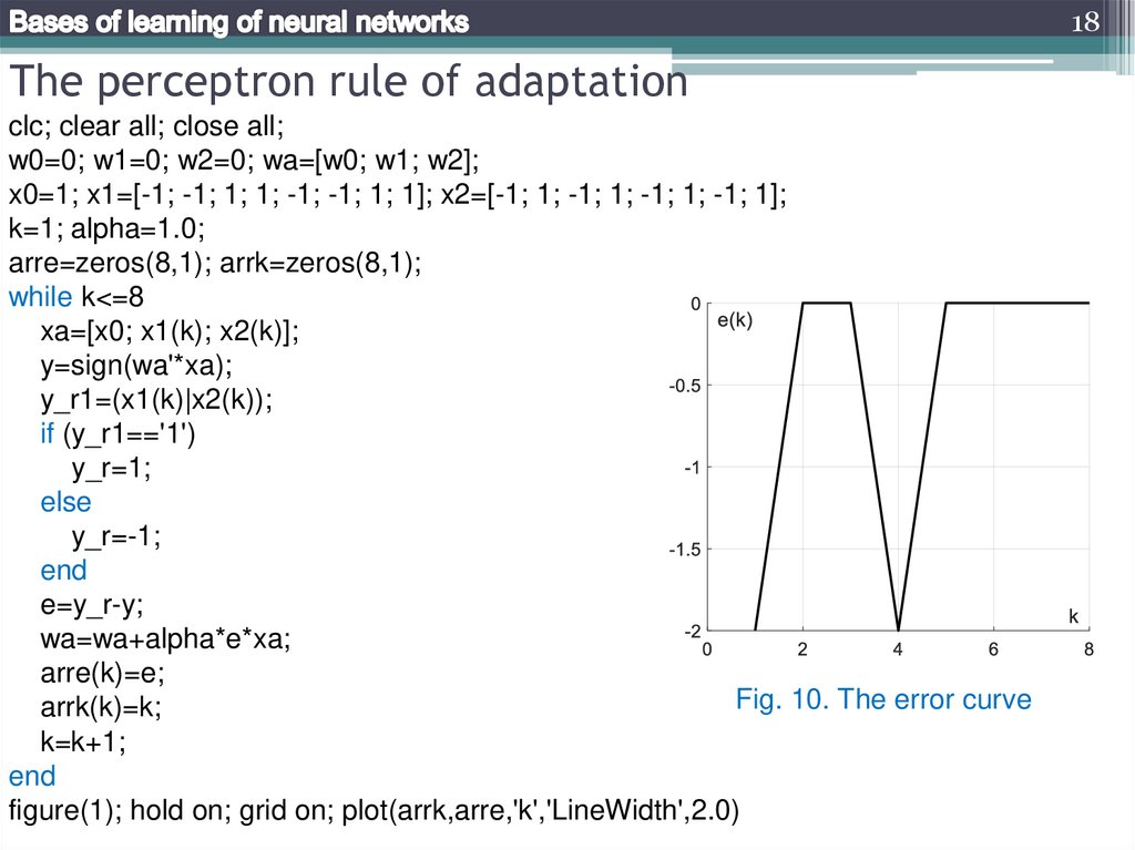
Let =1.0, initial value of vector wa is [0; 0; 0], number of the learning iterations k=8,
learning inputs are x0=[1; 1; 1; 1; 1; 1; 1; 1], x1=[-1; -1; 1; 1; -1; -1; 1; 1], x2=[-1; 1; -1; 1; 1; 1; -1; 1]. The learning error is shown in Fig. 2. The weights wa converge to
3
wa 1
1
(17)

18.

18
The perceptron rule of adaptation
clc; clear all; close all;
w0=0; w1=0; w2=0; wa=[w0; w1; w2];
x0=1; x1=[-1; -1; 1; 1; -1; -1; 1; 1]; x2=[-1; 1; -1; 1; -1; 1; -1; 1];
k=1; alpha=1.0;
arre=zeros(8,1); arrk=zeros(8,1);
while k<=8
xa=[x0; x1(k); x2(k)];
y=sign(wa'*xa);
y_r1=(x1(k)|x2(k));
if (y_r1=='1')
y_r=1;
else
y_r=-1;
end
e=y_r-y;
wa=wa+alpha*e*xa;
arre(k)=e;
Fig. 10. The error curve
arrk(k)=k;
k=k+1;
end
figure(1); hold on; grid on; plot(arrk,arre,'k','LineWidth',2.0)

19.

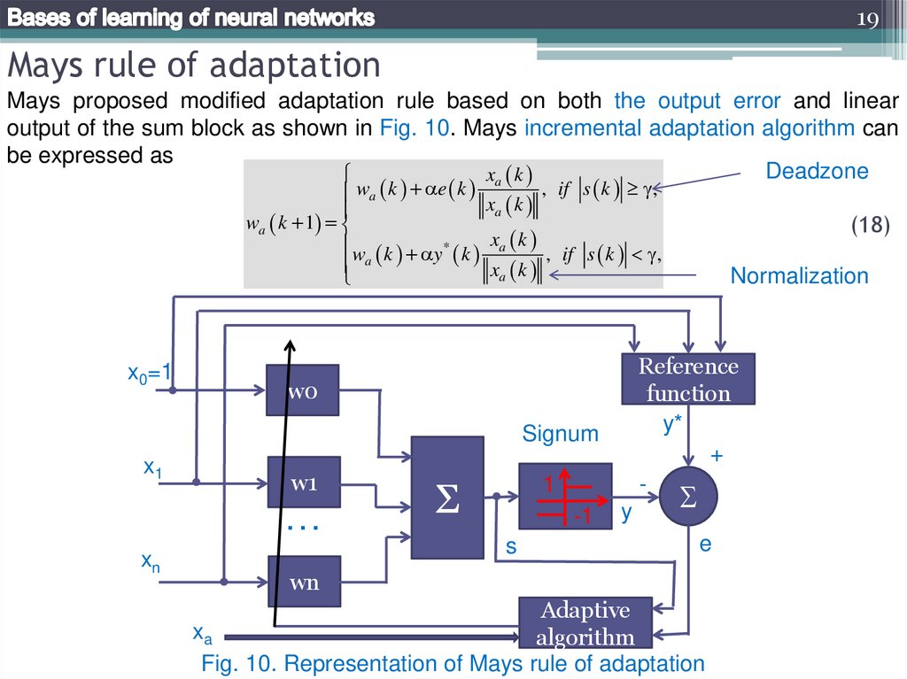
19
Mays rule of adaptation
Mays proposed modified adaptation rule based on both the output error and linear
output of the sum block as shown in Fig. 10. Mays incremental adaptation algorithm can
be expressed as
Deadzone
xa k
, if s k ,
wa k e k
xa k
wa k 1
w k y* k xa k , if s k ,
a
xa k
x0=1
w0
w1
…
xn
Σ
1
-1
s
Normalization
Reference
function
y*
+
-
Signum
x1
(18)
y
e
wn
Adaptive
xa
algorithm
Fig. 10. Representation of Mays rule of adaptation

20.

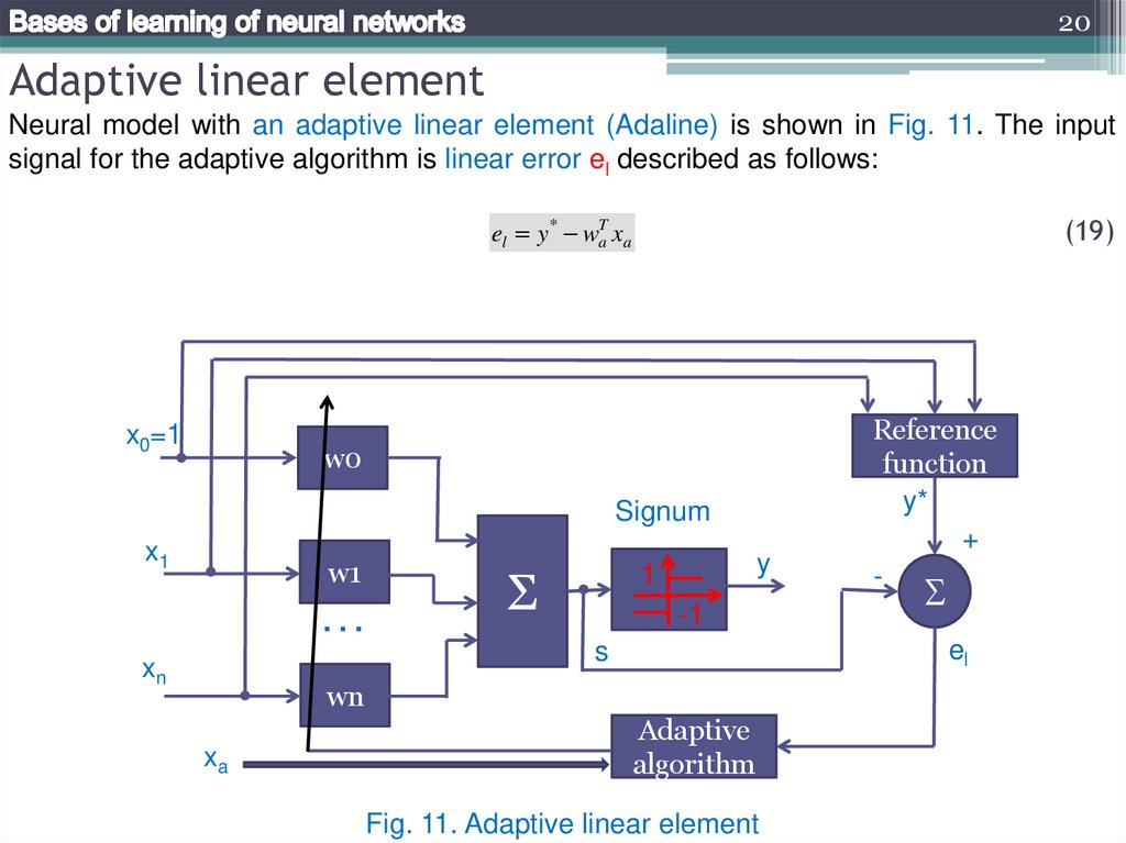
20
Adaptive linear element
Neural model with an adaptive linear element (Adaline) is shown in Fig. 11. The input
signal for the adaptive algorithm is linear error el described as follows:
(19)
el y* waT xa
x0=1
w0
Signum
x1
w1
…
xn
Σ
y
1
-1
el
s
wn
xa
Reference
function
y*
+
-
Adaptive
algorithm
Fig. 11. Adaptive linear element

21.

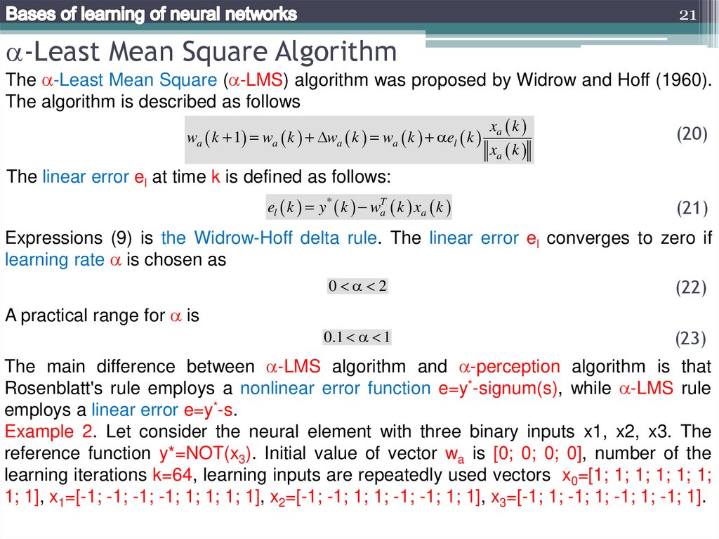
21
-Least Mean Square Algorithm
The -Least Mean Square ( -LMS) algorithm was proposed by Widrow and Hoff (1960).
The algorithm is described as follows
wa k 1 wa k wa k wa k el k
xa k
xa k
(20)
The linear error el at time k is defined as follows:
el k y* k waT k xa k
(21)
Expressions (9) is the Widrow-Hoff delta rule. The linear error el converges to zero if
learning rate is chosen as
0 2
(22)
0.1 1
(23)
A practical range for is
The main difference between -LMS algorithm and -perception algorithm is that
Rosenblatt's rule employs a nonlinear error function e=y*-signum(s), while -LMS rule
employs a linear error e=y*-s.
Example 2. Let consider the neural element with three binary inputs x1, x2, x3. The
reference function y*=NOT(x3). Initial value of vector wa is [0; 0; 0; 0], number of the
learning iterations k=64, learning inputs are repeatedly used vectors x0=[1; 1; 1; 1; 1; 1;
1; 1], x1=[-1; -1; -1; -1; 1; 1; 1; 1], x2=[-1; -1; 1; 1; -1; -1; 1; 1], x3=[-1; 1; -1; 1; -1; 1; -1; 1].

22.

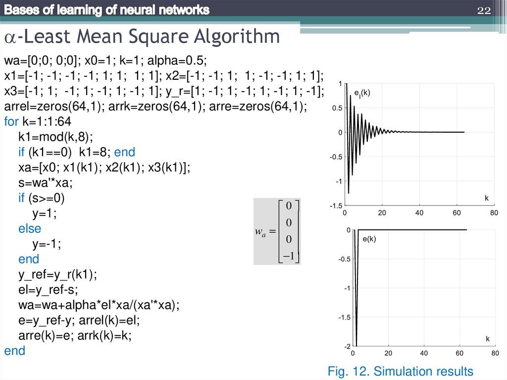
22
-Least Mean Square Algorithm
wa=[0;0; 0;0]; x0=1; k=1; alpha=0.5;
x1=[-1; -1; -1; -1; 1; 1; 1; 1]; x2=[-1; -1; 1; 1; -1; -1; 1; 1];
x3=[-1; 1; -1; 1; -1; 1; -1; 1]; y_r=[1; -1; 1; -1; 1; -1; 1; -1];
arrel=zeros(64,1); arrk=zeros(64,1); arre=zeros(64,1);
for k=1:1:64
k1=mod(k,8);
if (k1==0) k1=8; end
xa=[x0; x1(k1); x2(k1); x3(k1)];
s=wa'*xa;
if (s>=0)
0
y=1;
0
else
wa
0
y=-1;
1
end
y_ref=y_r(k1);
el=y_ref-s;
wa=wa+alpha*el*xa/(xa'*xa);
e=y_ref-y; arrel(k)=el;
arre(k)=e; arrk(k)=k;
end
Fig. 12. Simulation results

23.

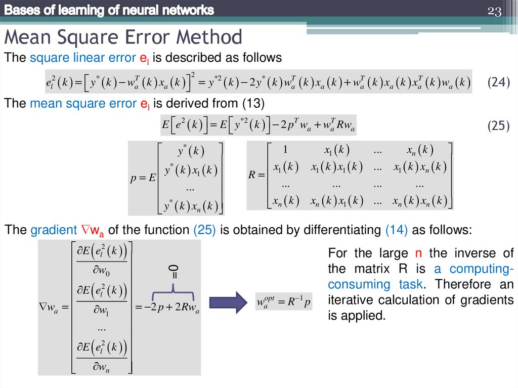
23
Mean Square Error Method
The square linear error el is described as follows
el2 k y* k waT k xa k y*2 k 2 y* k waT k xa k waT k xa k xaT k wa k
2
(24)
The mean square error el is derived from (13)
E e 2 k E y*2 k 2 pT wa waT Rwa
y* k
*
y k x1 k
p E
...
*
y k xn k
1
x k
R 1
...
xn k
x1 k
x1 k x1 k
...
xn k x1 k
(25)
...
xn k
... x1 k xn k
...
...
... xn k xn k
The gradient wa of the function (25) is obtained by differentiating (14) as follows:
=0
E el2 k
w
0
2
E el k
2 p 2 Rw
wa
w
a
1
...
2
E el k
wn
waopt R 1 p
For the large n the inverse of
the matrix R is a computingconsuming task. Therefore an
iterative calculation of gradients
is applied.

24.

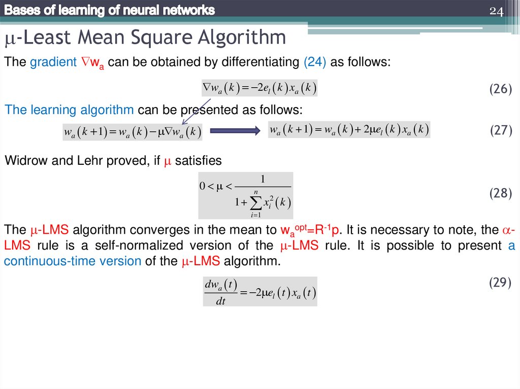
24
-Least Mean Square Algorithm
The gradient wa can be obtained by differentiating (24) as follows:
wa k 2el k xa k
(26)
The learning algorithm can be presented as follows:
wa k 1 wa k 2 el k xa k
wa k 1 wa k wa k
(27)
Widrow and Lehr proved, if satisfies
0
1
n
1 xi2 k
(28)
i 1
The -LMS algorithm converges in the mean to waopt=R-1p. It is necessary to note, the LMS rule is a self-normalized version of the -LMS rule. It is possible to present a
continuous-time version of the -LMS algorithm.
dwa t
dt
2 el t xa t
(29)

25.

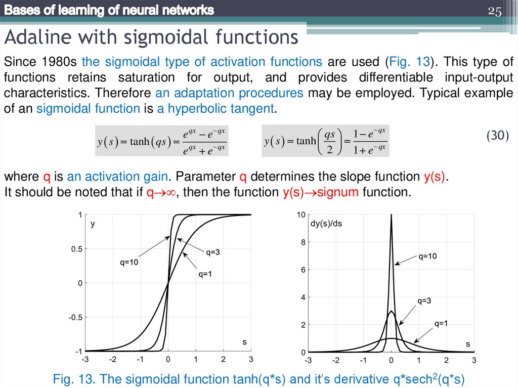
25
Adaline with sigmoidal functions
Since 1980s the sigmoidal type of activation functions are used (Fig. 13). This type of
functions retains saturation for output, and provides differentiable input-output
characteristics. Therefore an adaptation procedures may be employed. Typical example
of an sigmoidal function is a hyperbolic tangent.
e qx e qx
y s tanh qs qx
e e qx
qx
qs 1 e
y s tanh
qx
2 1 e
where q is an activation gain. Parameter q determines the slope function y(s).
It should be noted that if q , then the function y(s) signum function.
Fig. 13. The sigmoidal function tanh(q*s) and it’s derivative q*sech2(q*s)
(30)

26.

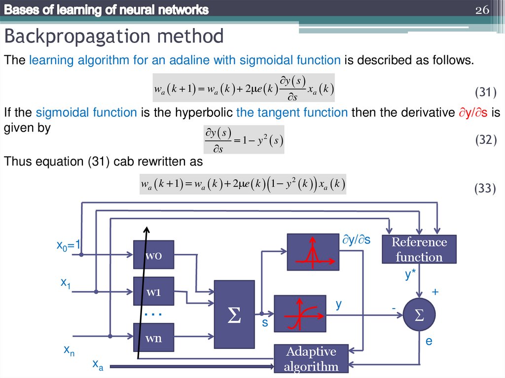
26
Backpropagation method
The learning algorithm for an adaline with sigmoidal function is described as follows.
wa k 1 wa k 2 e k
y s
s
xa k
(31)
If the sigmoidal function is the hyperbolic the tangent function then the derivative y/ s is
given by
y s
1 y2 s
(32)
s
Thus equation (31) cab rewritten as
wa k 1 wa k 2 e k 1 y 2 k xa k
y/ s
x0=1
w0
x1
w1
…
wn
xn
xa
Σ
y
s
Adaptive
algorithm
(33)
Reference
function
y*
+
-
e

27.

27
Problems
1. What are the advantages of automatic control over remote control?
2. What are the traits of the hard problems?
3. Draw the structure of the intelligent robot control system. What are the problems
solved by artificial intelligence?
4. Give the taxonomy of the artificial intelligence technologies.
5. Give a schematic diagram of a biological neuron. Explain the functions of dendrites,
axon, synapses, and soma.
6. Give a mathematical representation of a biological neuron. Explain the synaptic
operation and the somatic operation.
7. Give a structure and mathematical model of the threshold logic element. Illustrate
execution of logic operations AND, OR, NOT by the threshold logic element.
8. What is a linearly separable function? Give a geometric interpretation.
9. Give realization of XOR using a two-layered neural network.
10. Draw the structure of the parametric adaption of the neural threshold element.
Explain the element s of the structure. What are variables y*, e, xa?
11. Give the perception learning rule for discrete time k. Explain purpose of the
parameter .
12. Draw the block diagram of neuron with May rule of learning. Give mathematical
expressions for the rule.
13. Draw an adaptive linear element (Adaline). Explain variables s, el.

28.

28
Problems
1. Give the description of –Least Mean Square algorithm of Widow and Hoff. What is
main difference between –LMS and –perception rules?
2. Give the description of Mean Square Error Method. Wright the expression for the
gradient of wa in a matrix form.
3. Give the description of -Least Mean Square algorithm in an incremental form.
4. Give the expressions and graphs of the sigmoidal activation function. Explain the
purpose of parameter q?
5. Draw the diagram of the adaline with sigmoidal function and learning algorithm based
on the backpropagation method. Explain the diagram.