The Analysis of Competitive Markets. Chapter 9

1. Chapter 9

The Analysis of Competitive
Markets

2. Topics to be Discussed

Evaluating the Gains and Losses from
Government Policies
The Efficiency of a Competitive Market
Minimum Prices
Price Supports and Production Quotas
Import Quotas and Tariffs
The Impact of a Tax or Subsidy
©2005 Pearson Education, Inc.
Chapter 9
2

3. Consumer and Producer Surplus

When government controls price, some
people are better off
May be able to buy a good at a lower price
But what is the effect on society as a
whole?
Is total welfare higher or lower and by how
much?
A way to measure gains and losses from
government policies is needed
©2005 Pearson Education, Inc.
Chapter 9
3

4. Consumer and Producer Surplus

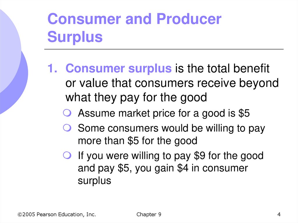
1. Consumer surplus is the total benefit
or value that consumers receive beyond
what they pay for the good
Assume market price for a good is $5
Some consumers would be willing to pay
more than $5 for the good
If you were willing to pay $9 for the good
and pay $5, you gain $4 in consumer
surplus
©2005 Pearson Education, Inc.
Chapter 9
4

5. Consumer and Producer Surplus

The demand curve shows the willingness
to pay for all consumers in the market
Consumer surplus can be measured by
the area between the demand curve and
the market price
Consumer surplus measures the total net
benefit to consumers
©2005 Pearson Education, Inc.
Chapter 9
5

6. Consumer and Producer Surplus

2. Producer surplus is the total benefit or
revenue that producers receive beyond
what it costs to produce a good
Some producers produce for less than
market price and would still produce at a
lower price
A producer might be willing to accept $3 for
the good but get $5 market price
Producer gains a surplus of $2
©2005 Pearson Education, Inc.
Chapter 9
6

7. Consumer and Producer Surplus

The supply curve shows the amount that
a producer is willing to take for a certain
amount of a good
Producer surplus can be measured by
the area between the supply curve and
the market price
Producer surplus measures the total net
benefit to producers
©2005 Pearson Education, Inc.
Chapter 9
7

8. Consumer and Producer Surplus

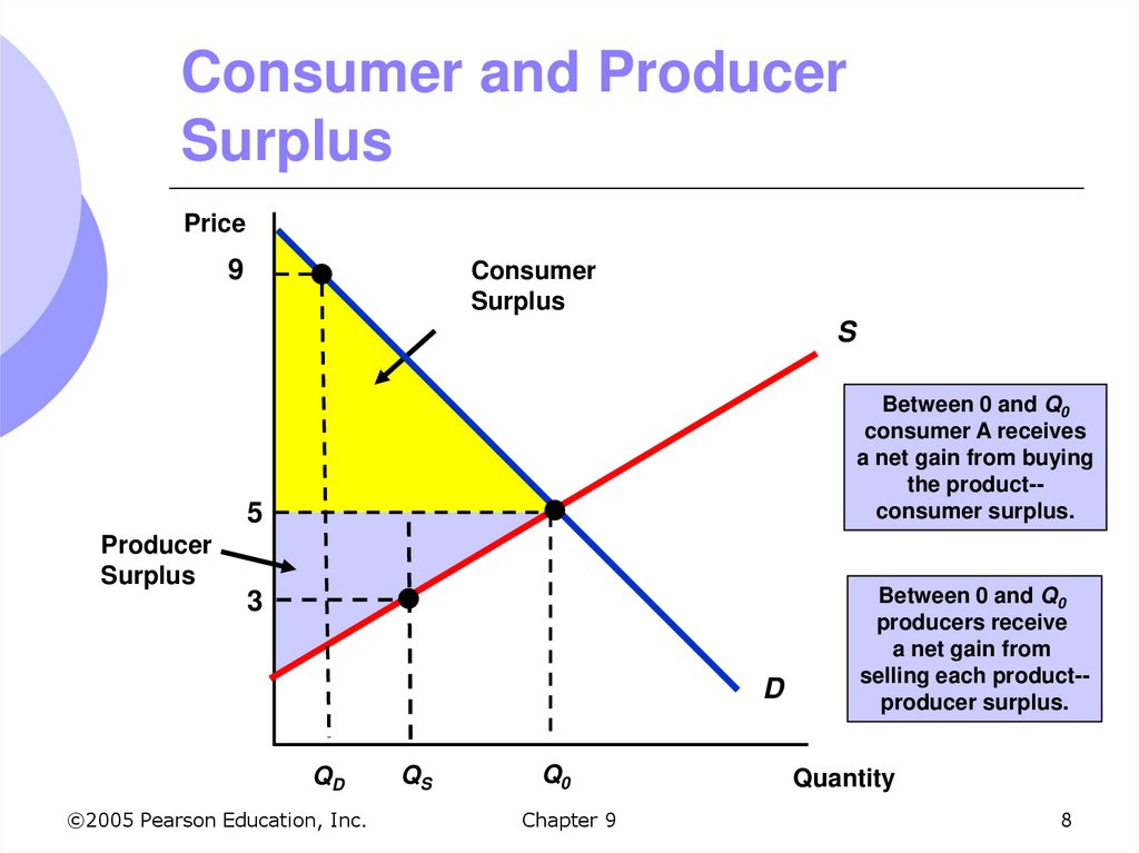
Price
9
Consumer
Surplus
S
Between 0 and Q0
consumer A receives
a net gain from buying
the product-consumer surplus.
5
Producer
Surplus
3
D
QD
©2005 Pearson Education, Inc.
QS
Q0
Chapter 9
Between 0 and Q0
producers receive
a net gain from
selling each product-producer surplus.
Quantity
8

9. Consumer and Producer Surplus

To determine the welfare effect of a
governmental policy, we can measure the
gain or loss in consumer and producer
surplus
Welfare Effects
Gains and losses to producers and
consumers
©2005 Pearson Education, Inc.
Chapter 9
9

10. Consumer and Producer Surplus

When government institutes a price
ceiling, the price of a good can’t go
above that price
With a binding price ceiling, producers
and consumers are affected
How much they are affected can be
determined by measuring changes in
consumer and producer surplus
©2005 Pearson Education, Inc.
Chapter 9
10

11. Consumer and Producer Surplus

When price is held too low, the quantity
demanded increases and quantity
supplied decreases
Some consumers are worse off because
they can no longer buy the good
Decrease in consumer surplus
Some consumers are better off because
they can buy it at a lower price
Increase in consumer surplus
©2005 Pearson Education, Inc.
Chapter 9
11

12. Consumer and Producer Surplus

Producers sell less at a lower price
Some producers are no longer in the
market
Both of these producer groups lose and
producer surplus decreases
The economy as a whole is worse off
since surplus that used to belong to
producers or consumers is simply gone
©2005 Pearson Education, Inc.
Chapter 9
12

13. Price Control and Surplus Changes

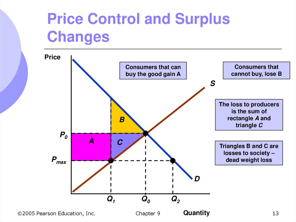
Price
Consumers that
cannot buy, lose B
Consumers that can
buy the good gain A
S
The loss to producers
is the sum of
rectangle A and
triangle C
B
P0
A
C
Triangles B and C are
losses to society –
dead weight loss
Pmax
D
Q1
©2005 Pearson Education, Inc.
Q0
Chapter 9
Q2
Quantity
13

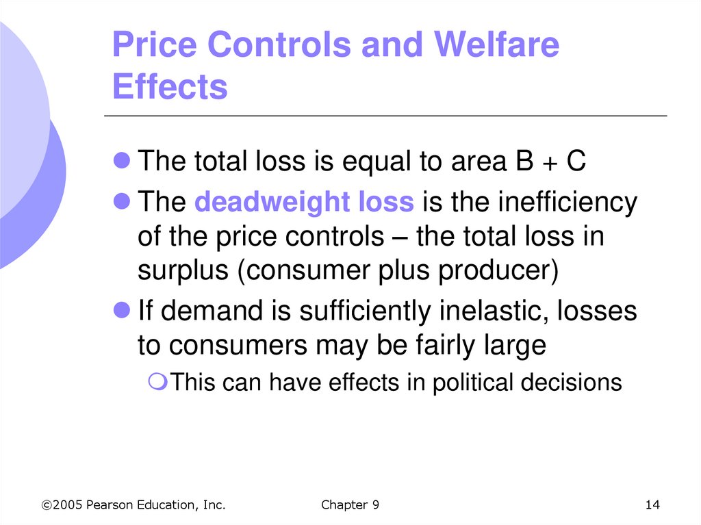
14. Price Controls and Welfare Effects

The total loss is equal to area B + C
The deadweight loss is the inefficiency
of the price controls – the total loss in
surplus (consumer plus producer)
If demand is sufficiently inelastic, losses
to consumers may be fairly large
This can have effects in political decisions
©2005 Pearson Education, Inc.
Chapter 9
14

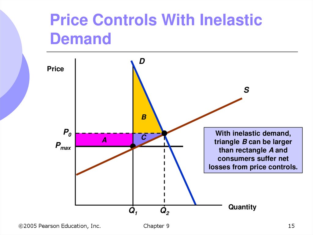
15. Price Controls With Inelastic Demand

D
Price
S
B
P0
Pmax
A
Q1
©2005 Pearson Education, Inc.
With inelastic demand,
triangle B can be larger
than rectangle A and
consumers suffer net
losses from price controls.
C
Q2
Chapter 9
Quantity
15

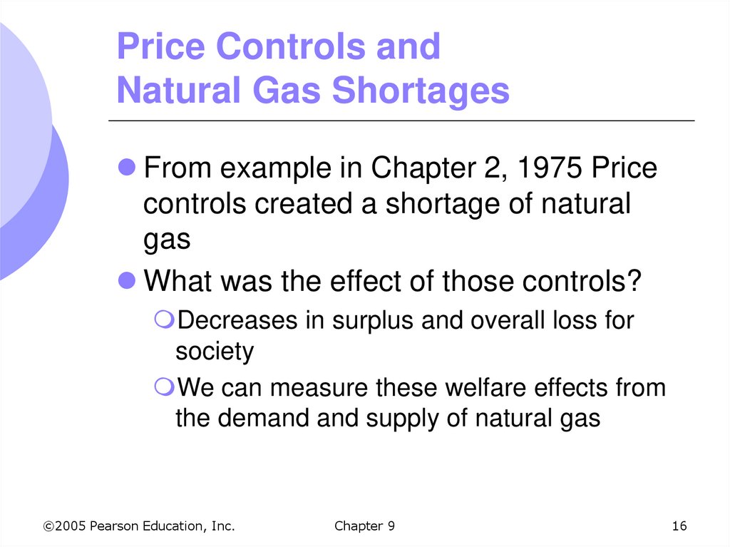
16. Price Controls and Natural Gas Shortages

From example in Chapter 2, 1975 Price
controls created a shortage of natural
gas
What was the effect of those controls?
Decreases in surplus and overall loss for
society
We can measure these welfare effects from
the demand and supply of natural gas
©2005 Pearson Education, Inc.
Chapter 9
16

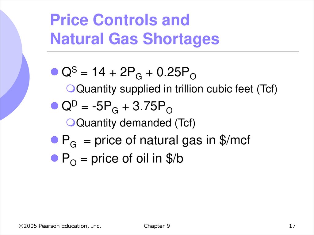
17. Price Controls and Natural Gas Shortages

QS = 14 + 2PG + 0.25PO
Quantity supplied in trillion cubic feet (Tcf)
QD = -5PG + 3.75PO
Quantity demanded (Tcf)
PG = price of natural gas in $/mcf
PO = price of oil in $/b
©2005 Pearson Education, Inc.
Chapter 9
17

18. Price Controls and Natural Gas Shortages

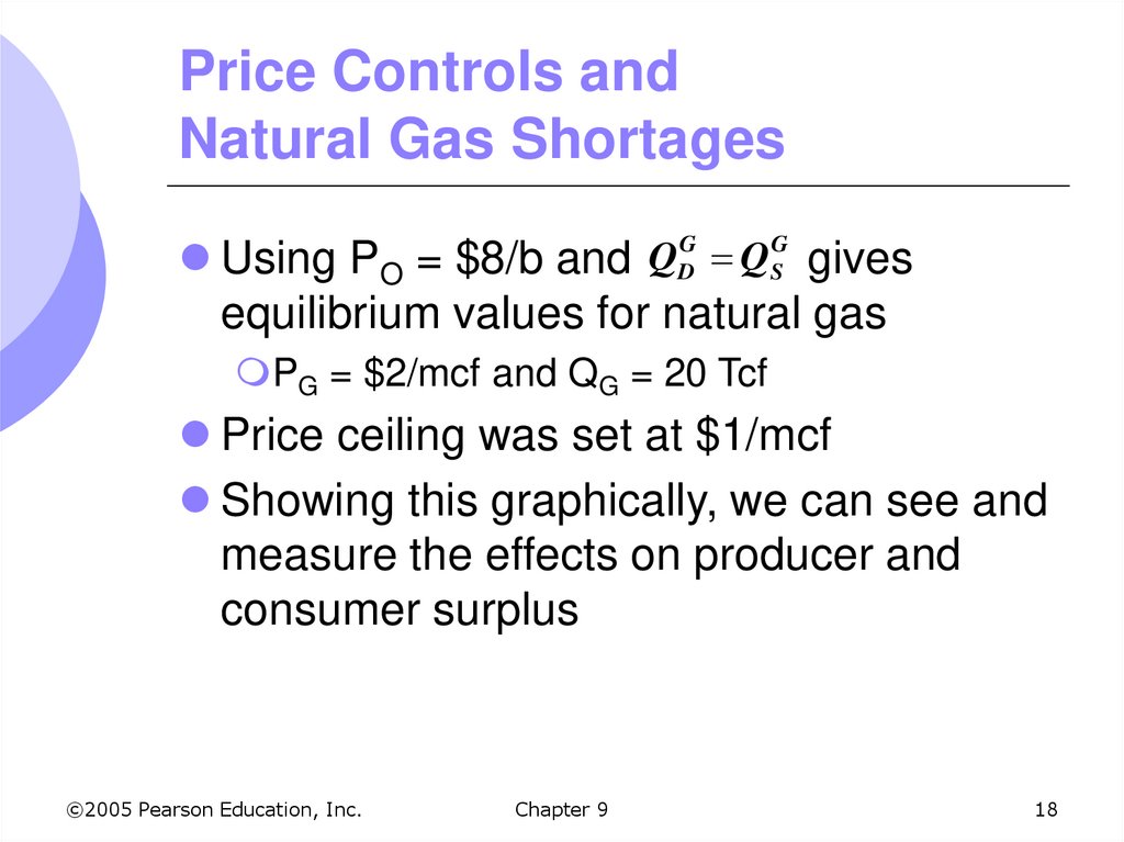
Using PO = $8/b and QDG QSG gives
equilibrium values for natural gas
PG = $2/mcf and QG = 20 Tcf
Price ceiling was set at $1/mcf
Showing this graphically, we can see and
measure the effects on producer and
consumer surplus
©2005 Pearson Education, Inc.
Chapter 9
18

19. Price Controls and Natural Gas Shortages

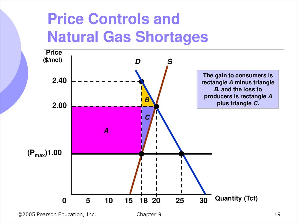
Price
($/mcf)
D
S
The gain to consumers is
rectangle A minus triangle
B, and the loss to
producers is rectangle A
plus triangle C.
2.40
B
2.00
C
A
(Pmax)1.00
0
5
©2005 Pearson Education, Inc.
10
15 18 20
Chapter 9
25
30 Quantity (Tcf)
19

20. Price Controls and Natural Gas Shortages

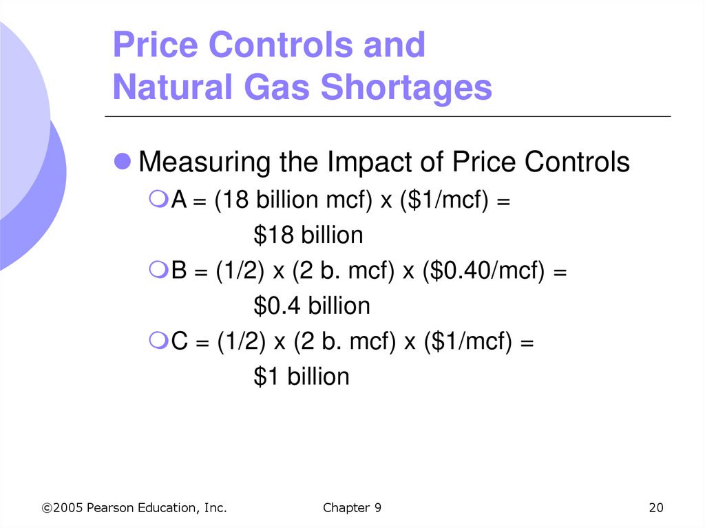
Measuring the Impact of Price Controls
A = (18 billion mcf) x ($1/mcf) =
$18 billion
B = (1/2) x (2 b. mcf) x ($0.40/mcf) =
$0.4 billion
C = (1/2) x (2 b. mcf) x ($1/mcf) =
$1 billion
©2005 Pearson Education, Inc.
Chapter 9
20

21. Price Controls and Natural Gas Shortages

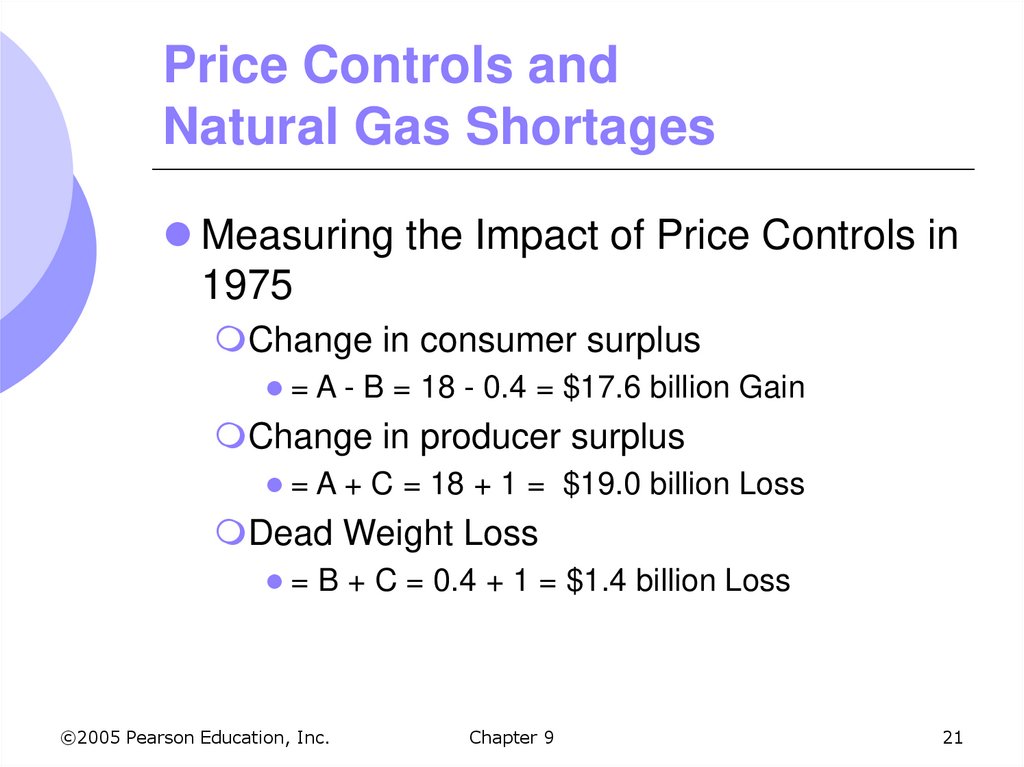
Measuring the Impact of Price Controls in
1975
Change in consumer surplus
= A - B = 18 - 0.4 = $17.6 billion Gain
Change in producer surplus
= A + C = 18 + 1 = $19.0 billion Loss
Dead Weight Loss
= B + C = 0.4 + 1 = $1.4 billion Loss
©2005 Pearson Education, Inc.
Chapter 9
21

22. The Efficiency of a Competitive Market

In the evaluation of markets, we often talk
about whether it reaches economic
efficiency
Maximization of aggregate consumer and
producer surplus
Policies such as price controls that cause
dead weight losses in society are said to
impose an efficiency cost on the
economy
©2005 Pearson Education, Inc.
Chapter 9
22

23. The Efficiency of a Competitive Market

If efficiency is the goal, then you can
argue that leaving markets alone is the
answer
However, sometimes market failures
occur
Prices fail to provide proper signals to
consumers and producers
Leads to inefficient unregulated competitive
market
©2005 Pearson Education, Inc.
Chapter 9
23

24. Types of Market Failures

1. Externalities
Costs or benefits that do not show up as
part of the market price (e.g. pollution)
Costs or benefits are external to the market
2. Lack of Information
Imperfect information prevents consumers
from making utility-maximizing decisions
Government intervention may be
desirable in these cases
©2005 Pearson Education, Inc.
Chapter 9
24

25. The Efficiency of a Competitive Market

Other than market failures, unregulated
competitive markets lead to economic
efficiency
What if the market is constrained to a
price higher than the economically
efficient equilibrium price?
©2005 Pearson Education, Inc.
Chapter 9
25

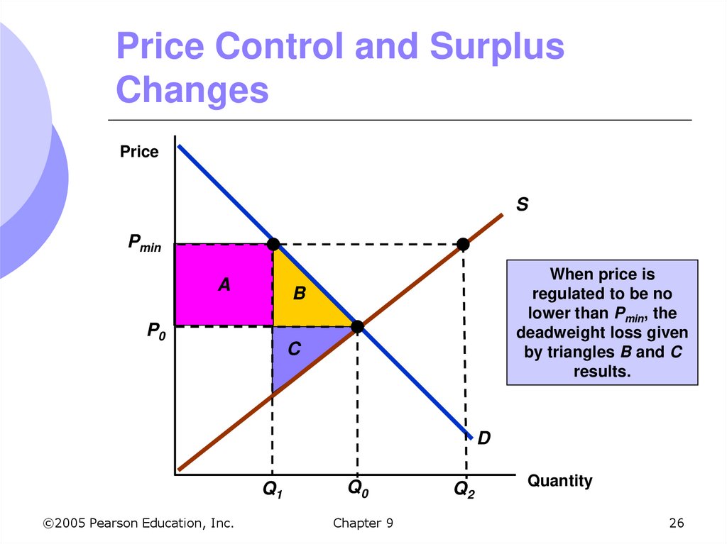
26. Price Control and Surplus Changes

Price
S
Pmin
A
When price is
regulated to be no
lower than Pmin, the
deadweight loss given
by triangles B and C
results.
B
P0
C
D
Q1
©2005 Pearson Education, Inc.
Q0
Chapter 9
Q2
Quantity
26

27. The Efficiency of a Competitive Market

Deadweight loss triangles B and C give a
good estimate of the efficiency cost of
policies that force price above or below
market clearing price
Measuring effects of government price
controls on the economy can be
estimated by measuring these two
triangles
©2005 Pearson Education, Inc.
Chapter 9
27

28. The Market for Human Kidneys

The 1984 National Organ Transplantation
Act prohibits the sale of organs for
transplantation
What has been the impact of the Act?
We can measure this using the supply
and demand for kidneys from estimated
data
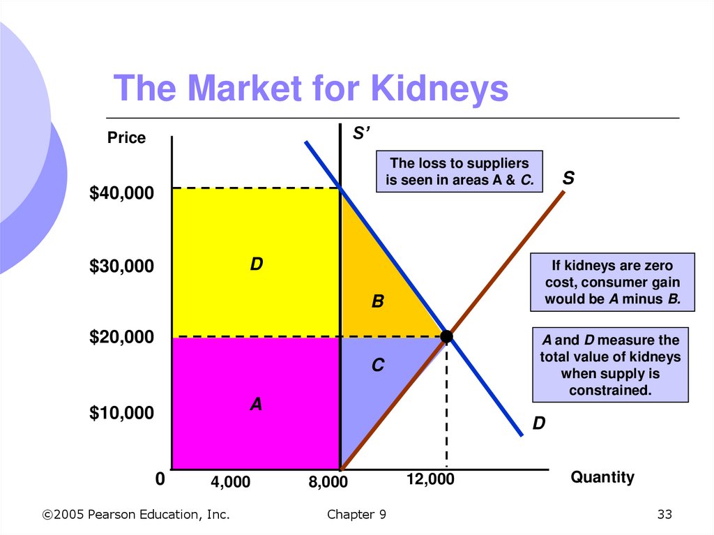
Supply: QS = 8,000 + 0.2P
Demand: QD = 16,000 - 0.2P
©2005 Pearson Education, Inc.
Chapter 9
28

29. The Market for Human Kidneys

Since the sale of organs is not allowed,
the amount available depends on the
amount donated
Supply of donated kidneys is limited to 8,000
The welfare effect of this supply
constraint can be analyzed using
consumer and producer surplus in the
kidney market
©2005 Pearson Education, Inc.
Chapter 9
29

30. The Market for Human Kidneys

Suppliers:
Those who supply them are not paid the
market price, estimated at $20,000
Loss of surplus equal to area A = $160 million
Some who would donate for the equilibrium
price do not donate in the current market
Loss of surplus equal to area C = $40 million
Total consumer loss of A + C = $200 million
©2005 Pearson Education, Inc.
Chapter 9
30

31. The Market for Human Kidneys

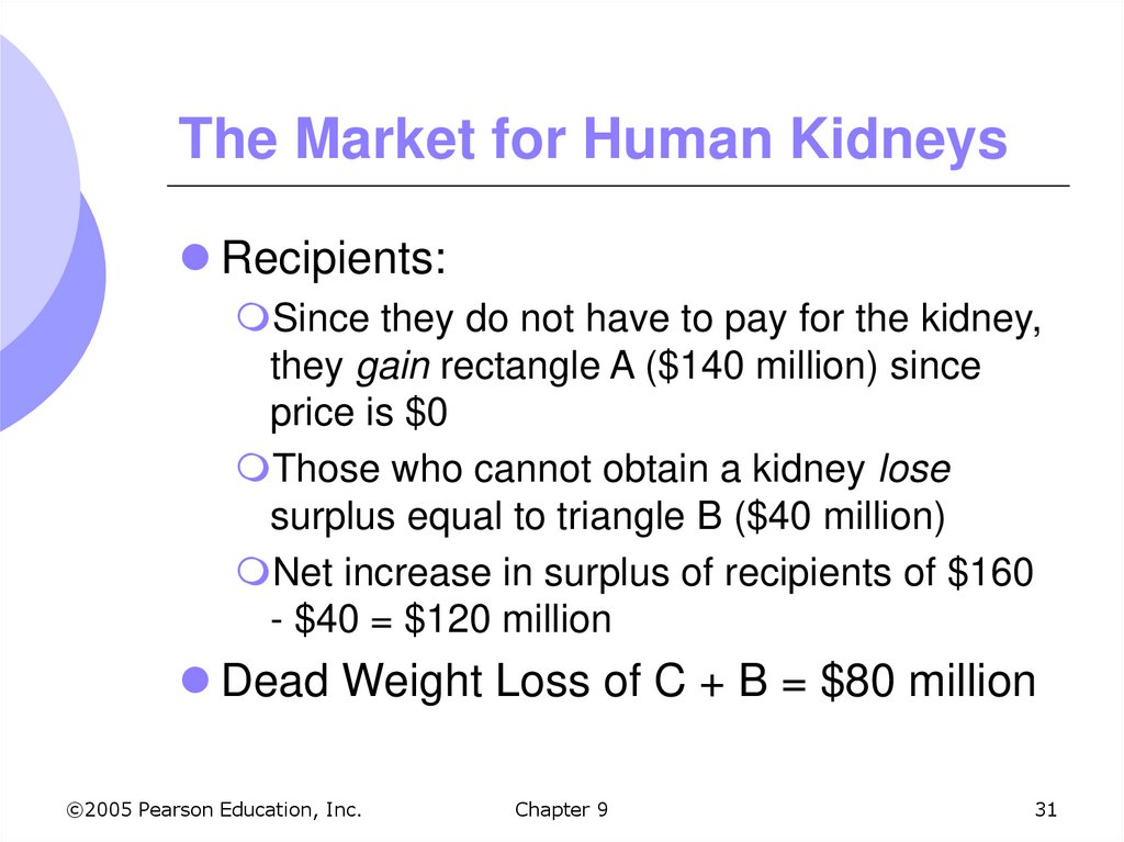
Recipients:
Since they do not have to pay for the kidney,
they gain rectangle A ($140 million) since
price is $0
Those who cannot obtain a kidney lose
surplus equal to triangle B ($40 million)
Net increase in surplus of recipients of $160
- $40 = $120 million
Dead Weight Loss of C + B = $80 million
©2005 Pearson Education, Inc.
Chapter 9
31

32. The Market for Human Kidneys

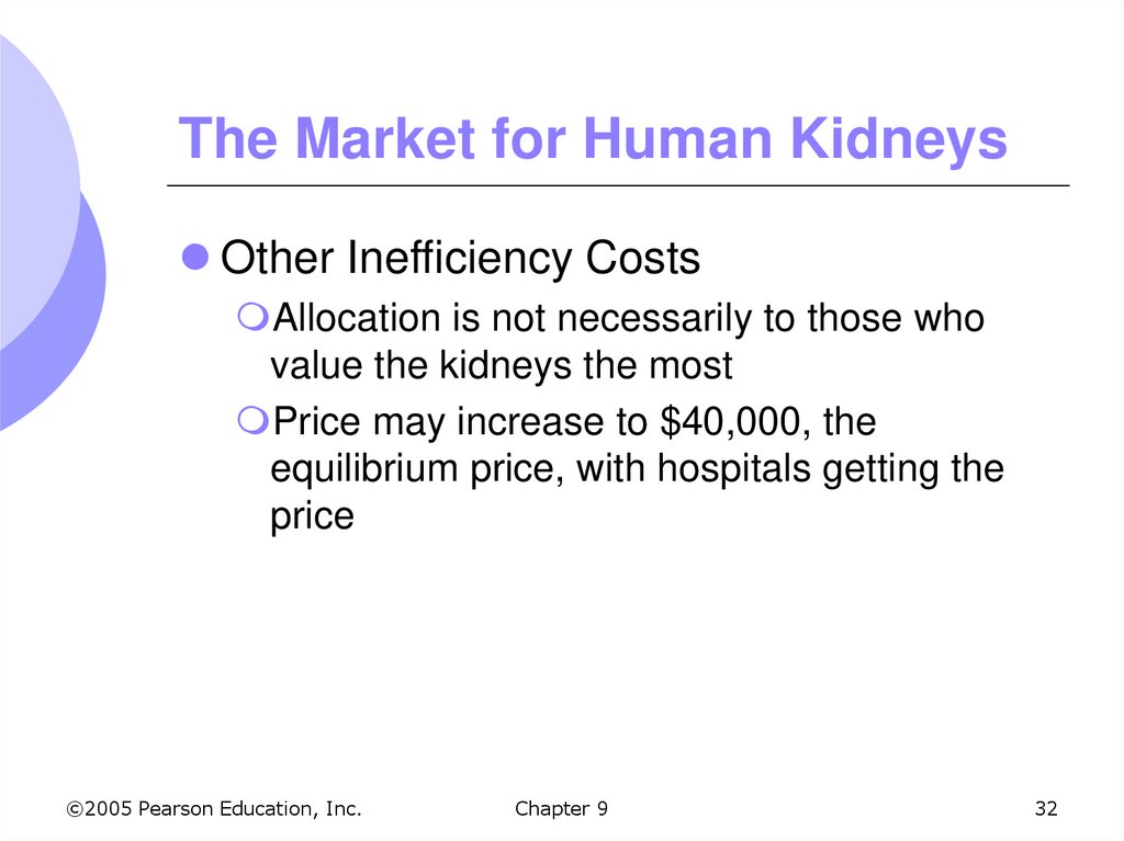
Other Inefficiency Costs
Allocation is not necessarily to those who
value the kidneys the most
Price may increase to $40,000, the
equilibrium price, with hospitals getting the
price
©2005 Pearson Education, Inc.
Chapter 9
32

33. The Market for Kidneys

S’
Price
The loss to suppliers
is seen in areas A & C.
$40,000
S
D
$30,000
If kidneys are zero
cost, consumer gain
would be A minus B.
B
$20,000
A and D measure the
total value of kidneys
when supply is
constrained.
C
A
$10,000
D
0
4,000
©2005 Pearson Education, Inc.
8,000
Chapter 9
12,000
Quantity
33

34. The Market for Human Kidneys

Arguments in favor of prohibiting the
sale of organs:
1. Imperfect information about donor’s health
and screening
2. Unfair to allocate according to the ability to
pay
Holding price below equilibrium will create
shortages
Organs versus artificial substitutes
©2005 Pearson Education, Inc.
Chapter 9
34

35. Minimum Prices

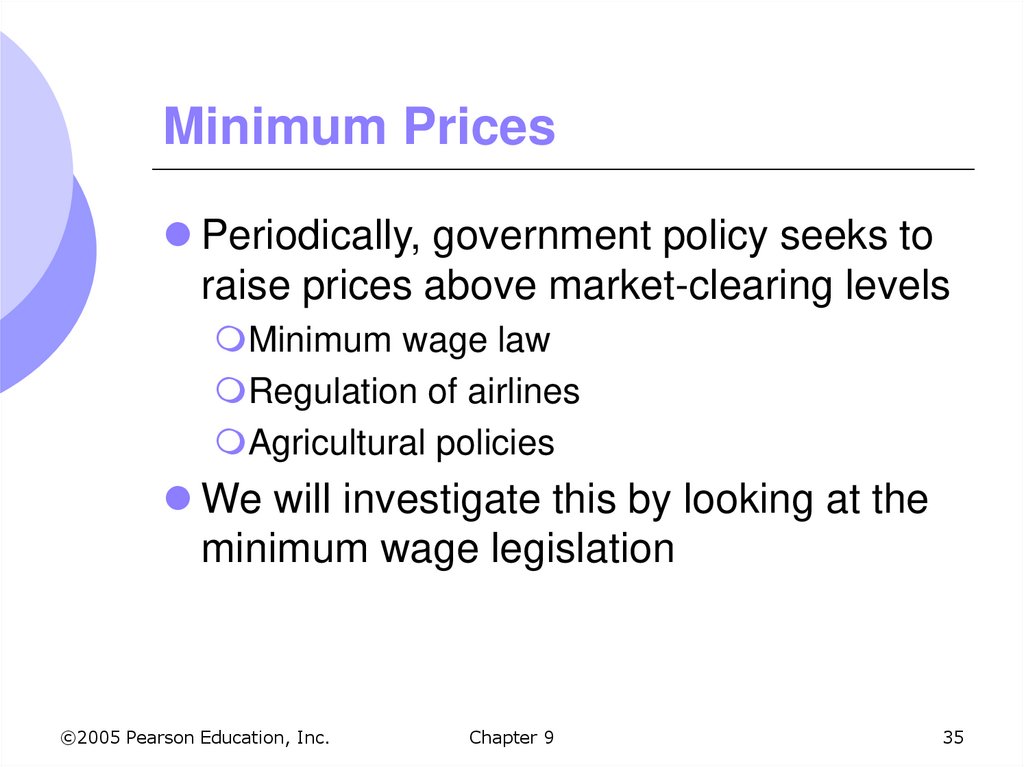
Periodically, government policy seeks to
raise prices above market-clearing levels
Minimum wage law
Regulation of airlines
Agricultural policies
We will investigate this by looking at the
minimum wage legislation
©2005 Pearson Education, Inc.
Chapter 9
35

36. Minimum Prices

When price is set above the market
clearing price:
Quantity demanded falls
Suppliers may, however, choose to increase
quantity supplied in face of higher prices
This causes additional producer losses equal
to the total cost of production above quantity
demanded
©2005 Pearson Education, Inc.
Chapter 9
36

37. Minimum Prices

Losses in consumer surplus are still the
same
Increased price leading to decreased
quantity equals area A
Those priced out of the market lose area B
Producer surplus similar
Increases from increased price for units sold
equal to A
Losses from drop in sales equal to C
©2005 Pearson Education, Inc.
Chapter 9
37

38. Minimum Prices

What if producers expand production to
Q2 from the increased price?
Since they only sell Q3, there is no revenue
to cover the additional production (Q2-Q3)
Supply curve measures MC of production so
total cost of additional production is area
under the supply curve for the increased
production (Q2-Q3) = area D
Total change in producer surplus = A – C – D
©2005 Pearson Education, Inc.
Chapter 9
38

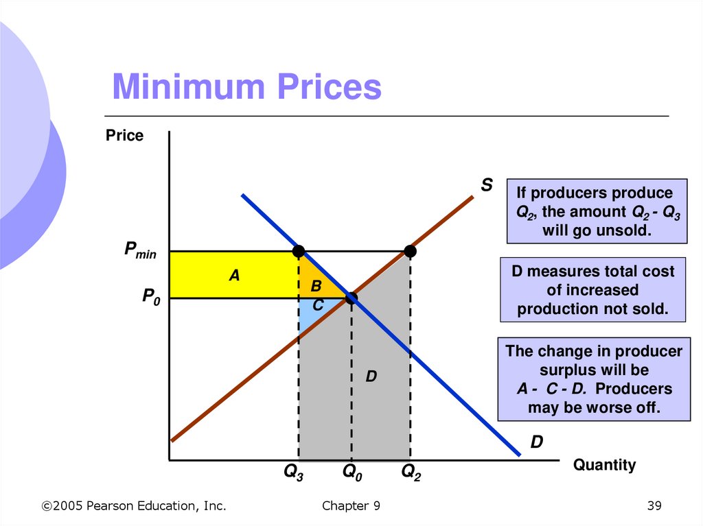
39. Minimum Prices

Price
S
If producers produce
Q2, the amount Q2 - Q3
will go unsold.
Pmin
A
D measures total cost
of increased
production not sold.
B
C
P0
The change in producer
surplus will be
A - C - D. Producers
may be worse off.
D
D
Q3
©2005 Pearson Education, Inc.
Q0
Chapter 9
Q2
Quantity
39

40. Minimum Wages

Wage is set higher than market clearing
wage
Decreased quantity of workers
demanded
Those workers hired receive higher
wages
Unemployment results, since not
everyone who wants to work at the new
wage can
©2005 Pearson Education, Inc.
Chapter 9
40

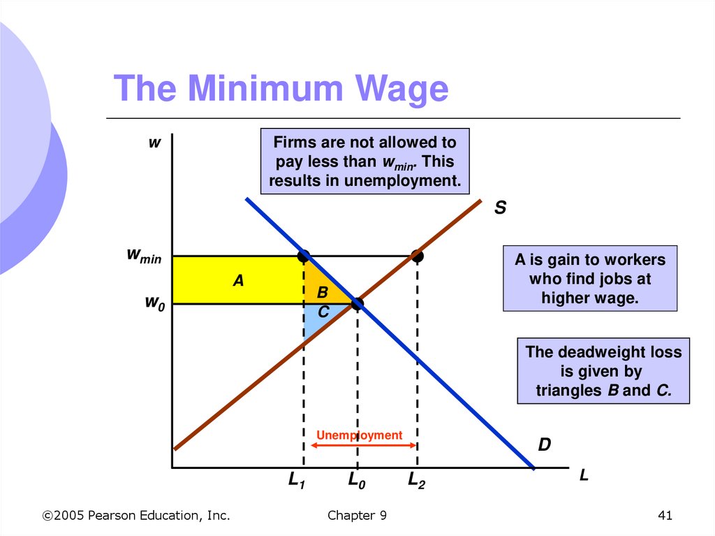
41. The Minimum Wage

Firms are not allowed to
pay less than wmin. This
results in unemployment.
w
S
wmin
A
A is gain to workers
who find jobs at
higher wage.
B
C
w0
The deadweight loss
is given by
triangles B and C.
Unemployment
L1
©2005 Pearson Education, Inc.
L0
Chapter 9
D
L2
L
41

42. Airline Regulation

Before 1970, the airline industry was
heavily regulated by the Civil Aeronautics
Board (CAB)
During 1976-1981, the airline industry in
the U.S. changed dramatically as
deregulation led to major changes
Some airlines merged or went out of
business as new airlines entered the
industry
©2005 Pearson Education, Inc.
Chapter 9
42

43. Airline Regulation

Although prices in the industry fell
considerably (helping consumers), profits
did not.
Regulation caused significant inefficiencies
and artificially high costs
We can show the effects of this
regulation by looking at the effects on
surplus from the controlled prices
©2005 Pearson Education, Inc.
Chapter 9
43

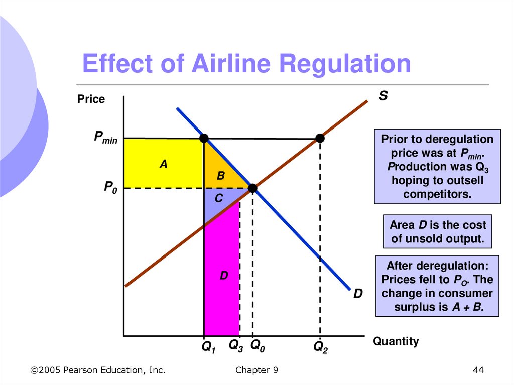
44. Effect of Airline Regulation

S
Price
Pmin
Prior to deregulation
price was at Pmin.
Production was Q3
hoping to outsell
competitors.
A
P0
B
C
Area D is the cost
of unsold output.
D
D
Q1 Q3 Q 0
©2005 Pearson Education, Inc.
Chapter 9
Q2
After deregulation:
Prices fell to PO. The
change in consumer
surplus is A + B.
Quantity
44

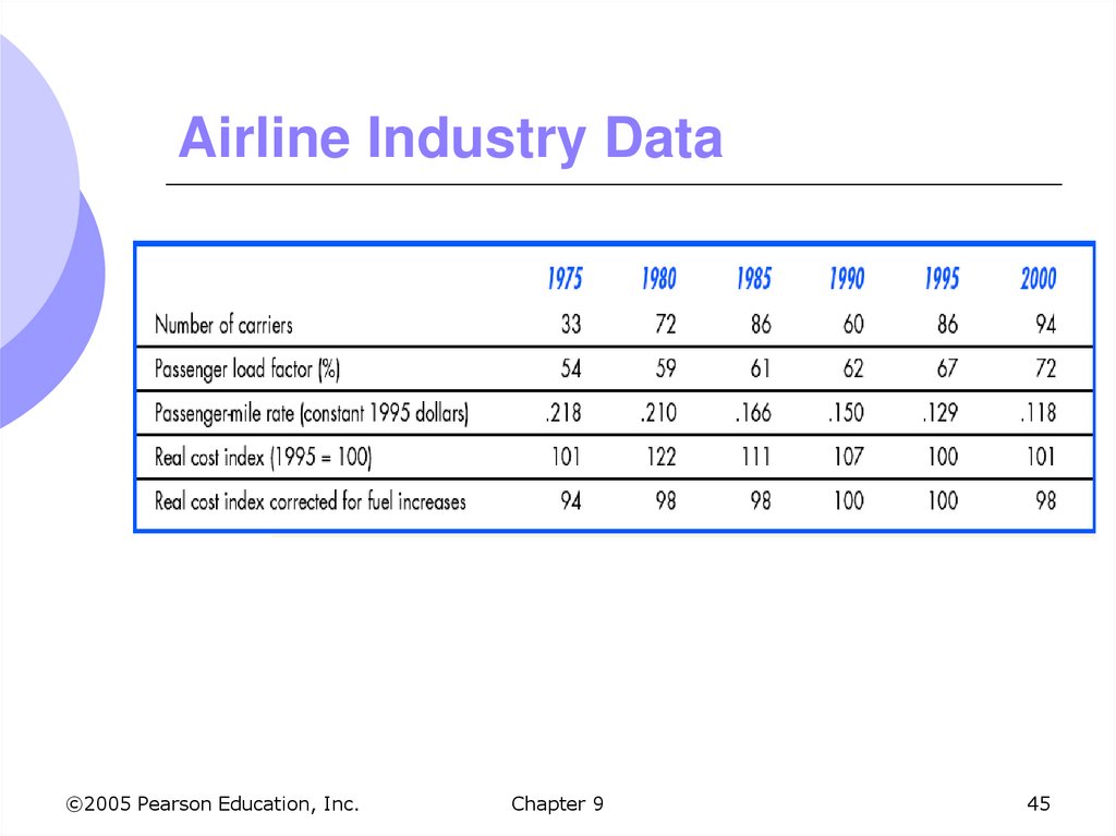
45. Airline Industry Data

©2005 Pearson Education, Inc.
Chapter 9
45

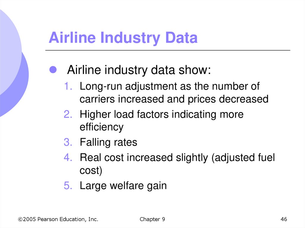
46. Airline Industry Data

Airline industry data show:
1. Long-run adjustment as the number of
carriers increased and prices decreased
2. Higher load factors indicating more
efficiency
3. Falling rates
4. Real cost increased slightly (adjusted fuel
cost)
5. Large welfare gain
©2005 Pearson Education, Inc.
Chapter 9
46

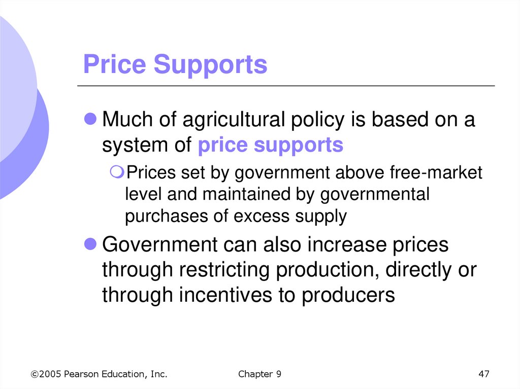
47. Price Supports

Much of agricultural policy is based on a
system of price supports
Prices set by government above free-market
level and maintained by governmental
purchases of excess supply
Government can also increase prices
through restricting production, directly or
through incentives to producers
©2005 Pearson Education, Inc.
Chapter 9
47

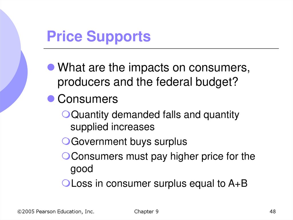
48. Price Supports

What are the impacts on consumers,
producers and the federal budget?
Consumers
Quantity demanded falls and quantity
supplied increases
Government buys surplus
Consumers must pay higher price for the
good
Loss in consumer surplus equal to A+B
©2005 Pearson Education, Inc.
Chapter 9
48

49. Price Supports

Producers
Gain since they are selling more at a higher
price
Producer surplus increases by A+B+D
Government
Cost of buying the surplus, which is funded
by taxes, so indirect cost on consumers
Cost to government = (Q2-Q1)PS
©2005 Pearson Education, Inc.
Chapter 9
49

50. Price Supports

Government may be able to “dump” some of the
goods in the foreign markets
Hurts domestic producers that government is trying to
help in the first place
Total welfare effect of policy
CS + PS – Govt. cost = D – (Q2-Q1)PS
Society is worse off overall
Less costly to simply give farmers the money
©2005 Pearson Education, Inc.
Chapter 9
50

51. Price Supports

Price
S
Qg
Ps
A
P0
To maintain a price Ps
the government buys
quantity Qg .
D
B
Net Loss to
society is E + B.
D + Qg
E
D
Q1
©2005 Pearson Education, Inc.
Q0
Q2
Chapter 9
Quantity
51

52. Production Quotas

The government can also cause the price
of a good to rise by reducing supply
Limitations of taxi medallions in New York
City
Limitation of required liquor licenses for
restaurants
©2005 Pearson Education, Inc.
Chapter 9
52

53. Supply Restrictions

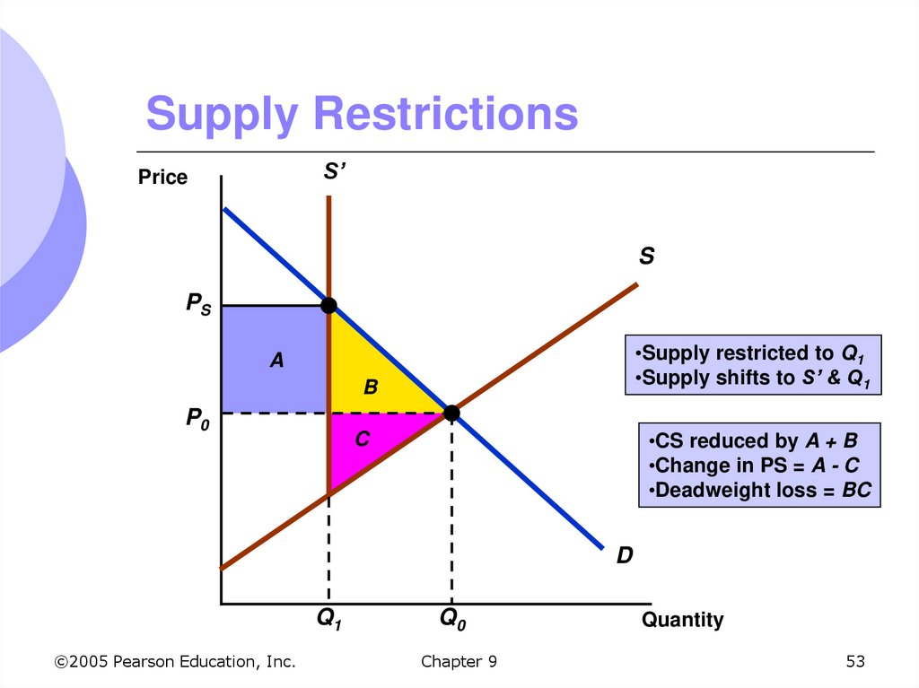
S’
Price
S
PS
•Supply restricted to Q1
•Supply shifts to S’ & Q1
A
B
P0
•CS reduced by A + B
•Change in PS = A - C
•Deadweight loss = BC
C
D
Q1
©2005 Pearson Education, Inc.
Q0
Chapter 9
Quantity
53

54. Supply Restrictions

Incentive Programs
US agricultural policy uses production
incentives instead of direct quotas
Government gives farmers financial
incentives to restrict supply
Acreage limitation programs
Quantity decreases and price increases for
the crop
©2005 Pearson Education, Inc.
Chapter 9
54

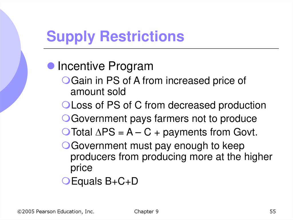
55. Supply Restrictions

Incentive Program
Gain in PS of A from increased price of
amount sold
Loss of PS of C from decreased production
Government pays farmers not to produce
Total PS = A – C + payments from Govt.
Government must pay enough to keep
producers from producing more at the higher
price
Equals B+C+D
©2005 Pearson Education, Inc.
Chapter 9
55

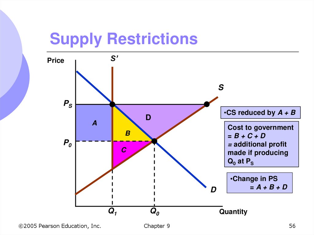
56. Supply Restrictions

S’
Price
S
PS
•CS reduced by A + B
D
A
Cost to government
=B+C+D
= additional profit
made if producing
Q0 at PS
B
P0
C
D
Q1
©2005 Pearson Education, Inc.
Q0
Chapter 9
•Change in PS
=A+B+D
Quantity
56

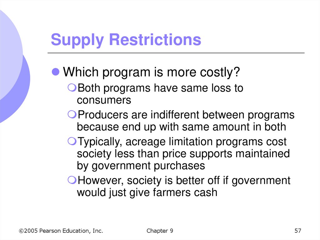
57. Supply Restrictions

Which program is more costly?
Both programs have same loss to
consumers
Producers are indifferent between programs
because end up with same amount in both
Typically, acreage limitation programs cost
society less than price supports maintained
by government purchases
However, society is better off if government
would just give farmers cash
©2005 Pearson Education, Inc.
Chapter 9
57

58. Supporting the Price of Wheat

From previous example, the supply and
demand for wheat in 1981 was
Supply: QS = 1,800 + 240P
Demand: QD = 3,550 - 266P
Equilibrium price and quantity was $3.46 and
2,630 million bushels
Government raised the price to $3.70
through government purchases
©2005 Pearson Education, Inc.
Chapter 9
58

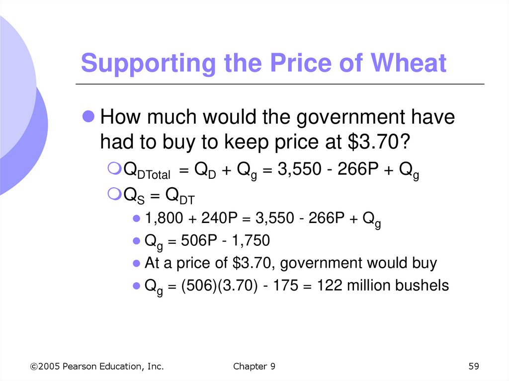
59. Supporting the Price of Wheat

How much would the government have
had to buy to keep price at $3.70?
QDTotal = QD + Qg = 3,550 - 266P + Qg
QS = QDT
1,800 + 240P = 3,550 - 266P + Qg
Qg = 506P - 1,750
At a price of $3.70, government would buy
Qg = (506)(3.70) - 175 = 122 million bushels
©2005 Pearson Education, Inc.
Chapter 9
59

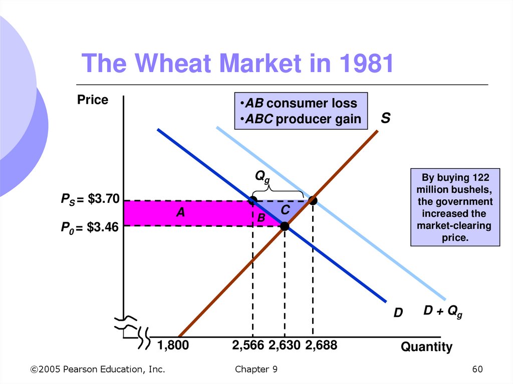
60. The Wheat Market in 1981

Price
•AB consumer loss
•ABC producer gain
S
Qg
PS = $3.70
A
P0 = $3.46
B
By buying 122
million bushels,
the government
increased the
market-clearing
price.
C
D
1,800
©2005 Pearson Education, Inc.
2,566 2,630 2,688
Chapter 9
D + Qg
Quantity
60

61. Supporting the Price of Wheat

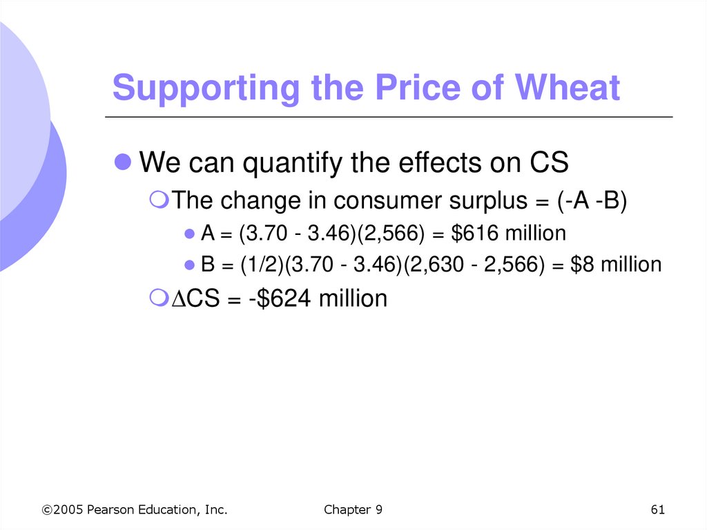
We can quantify the effects on CS
The change in consumer surplus = (-A -B)
A = (3.70 - 3.46)(2,566) = $616 million
B = (1/2)(3.70 - 3.46)(2,630 - 2,566) = $8 million
CS = -$624 million
©2005 Pearson Education, Inc.
Chapter 9
61

62. Supporting the Price of Wheat

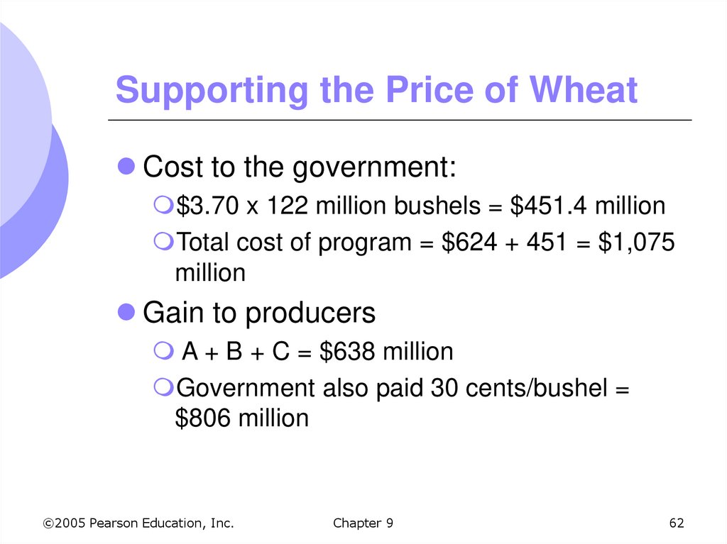
Cost to the government:
$3.70 x 122 million bushels = $451.4 million
Total cost of program = $624 + 451 = $1,075
million
Gain to producers
A + B + C = $638 million
Government also paid 30 cents/bushel =
$806 million
©2005 Pearson Education, Inc.
Chapter 9
62

63. Supporting the Price of Wheat

In 1985, the situation became worse
Export demand fell and the market clearing
price of wheat fell to $1.80/bushel
Equilibrium quantity was 2231
The actual price, however, was $3.20
To keep price at $3.20, the government had
to purchase excess wheat
Government also imposed a production
quota of about 2425 million bushels
©2005 Pearson Education, Inc.
Chapter 9
63

64. Supporting the Price of Wheat

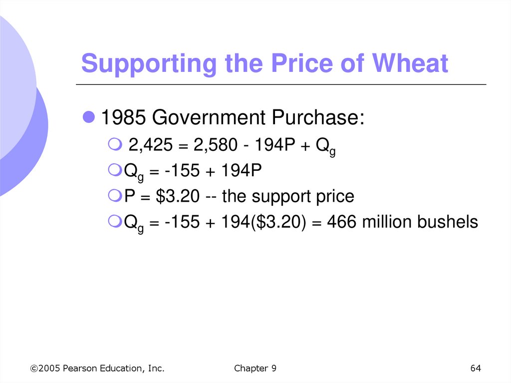
1985 Government Purchase:
2,425 = 2,580 - 194P + Qg
Qg = -155 + 194P
P = $3.20 -- the support price
Qg = -155 + 194($3.20) = 466 million bushels
©2005 Pearson Education, Inc.
Chapter 9
64

65. The Wheat Market in 1985

Price
S
’
S
Qg
To increase the
price to $3.20, the
government bought
466 million bushels
and imposed
a production quota
of 2,425 bushels.
PS = $3.20
P0 = $1.80
D
1,800 1,959
©2005 Pearson Education, Inc.
2,232 2,425
Chapter 9
D + Qg
Quantity
65

66. Supporting the Price of Wheat

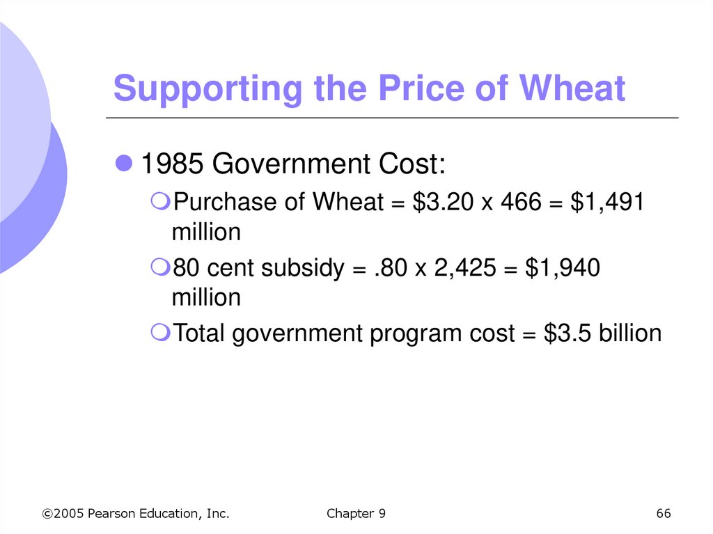
1985 Government Cost:
Purchase of Wheat = $3.20 x 466 = $1,491
million
80 cent subsidy = .80 x 2,425 = $1,940
million
Total government program cost = $3.5 billion
©2005 Pearson Education, Inc.
Chapter 9
66

67. Supporting the Price of Wheat

In 1996, Congress passed the Freedom
to Farm law
Goal was to reduce the role of government
and make agriculture more market-oriented
Eliminated production quotas, gradually
reduced government purchases and
subsidies through 2003
©2005 Pearson Education, Inc.
Chapter 9
67

68. Supporting the Price of Wheat

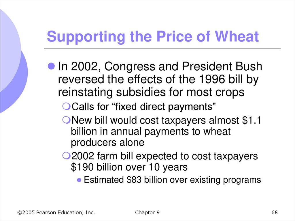
In 2002, Congress and President Bush
reversed the effects of the 1996 bill by
reinstating subsidies for most crops
Calls for “fixed direct payments”
New bill would cost taxpayers almost $1.1
billion in annual payments to wheat
producers alone
2002 farm bill expected to cost taxpayers
$190 billion over 10 years
Estimated $83 billion over existing programs
©2005 Pearson Education, Inc.
Chapter 9
68

69. Import Quotas and Tariffs

Many countries use import quotas and
tariffs to keep the domestic price of a
product above world levels
Import quotas: Limit on the quantity of a
good that can be imported
Tariff: Tax on an imported good
This allows domestic producers to enjoy
higher profits
Cost to consumers is high
©2005 Pearson Education, Inc.
Chapter 9
69

70. Import Quotas and Tariffs

With lower world price, domestic
consumers have incentive to purchase
from abroad
Domestic price falls to world price and
imports equal difference between quantity
supplied and quantity demanded
Domestic industry might convince
government to protect industry by
eliminating imports
Quota of zero or high tariff
©2005 Pearson Education, Inc.
Chapter 9
70

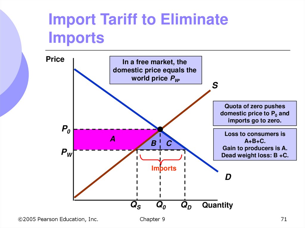
71. Import Tariff to Eliminate Imports

Price
In a free market, the
domestic price equals the
world price PW.
S
Quota of zero pushes
domestic price to P0 and
imports go to zero.
P0
A
B
Loss to consumers is
A+B+C.
Gain to producers is A.
Dead weight loss: B +C.
C
PW
Imports
D
QS
©2005 Pearson Education, Inc.
Q0
Chapter 9
QD
Quantity
71

72. Import Tariff (General Case)

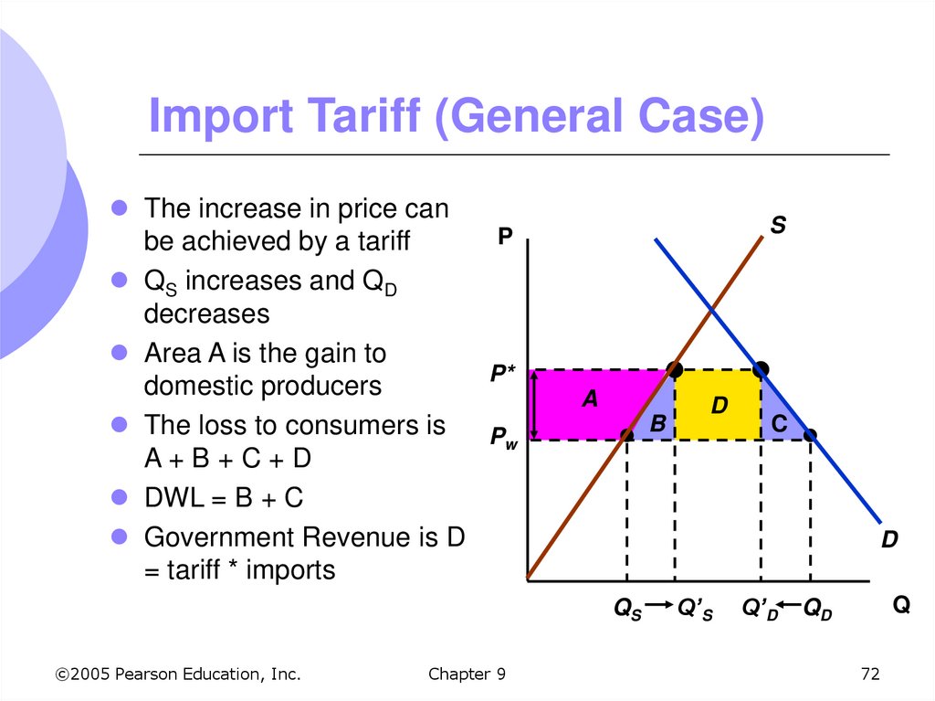
The increase in price can
P
be achieved by a tariff
QS increases and QD
decreases
Area A is the gain to
P*
domestic producers
The loss to consumers is
Pw
A+B+C+D
DWL = B + C
Government Revenue is D
= tariff * imports
S
A
B
Chapter 9
C
D
QS
©2005 Pearson Education, Inc.
D
Q’S
Q’D
Q
QD
72

73. Import Quota (General Case)

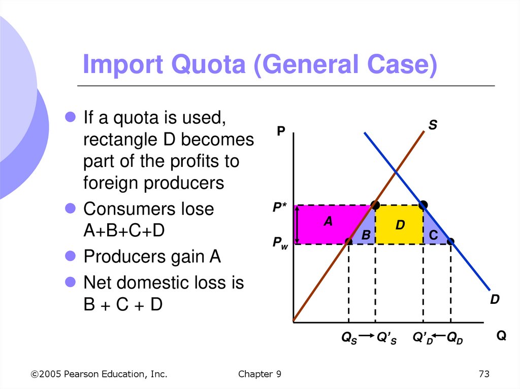
If a quota is used,
rectangle D becomes
part of the profits to
foreign producers
Consumers lose
A+B+C+D
Producers gain A
Net domestic loss is
B+C+D
S
P
P*
A
B
Pw
Chapter 9
C
D
QS
©2005 Pearson Education, Inc.
D
Q’S
Q’D
Q
QD
73

74. The Sugar Quota Example

The world price of sugar has been as low as 4
cents per pound, while in the U.S. the price has
been 20-25 cents per pound
Sugar quotas have protected the sugar industry
but driven up prices
Domestic producers have been better off and so
have some foreign producers that have quota
rights
Consumers are worse off
©2005 Pearson Education, Inc.
Chapter 9
74

75. The Sugar Quota Example

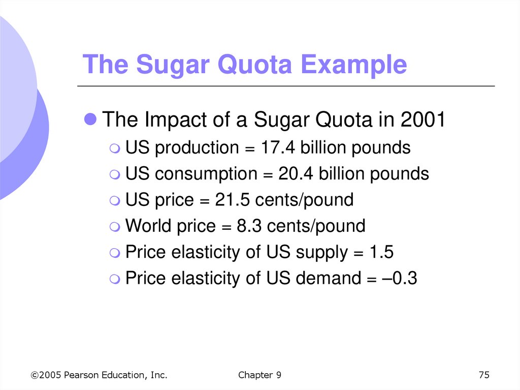
The Impact of a Sugar Quota in 2001
US production = 17.4 billion pounds
US consumption = 20.4 billion pounds
US price = 21.5 cents/pound
World price = 8.3 cents/pound
Price elasticity of US supply = 1.5
Price elasticity of US demand = –0.3
©2005 Pearson Education, Inc.
Chapter 9
75

76. Impact of Sugar Quota

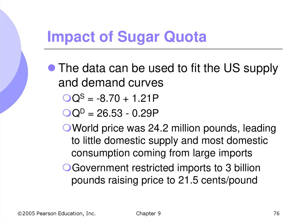
The data can be used to fit the US supply
and demand curves
QS = -8.70 + 1.21P
QD = 26.53 - 0.29P
World price was 24.2 million pounds, leading
to little domestic supply and most domestic
consumption coming from large imports
Government restricted imports to 3 billion
pounds raising price to 21.5 cents/pound
©2005 Pearson Education, Inc.
Chapter 9
76

77. Sugar Quota in 1997

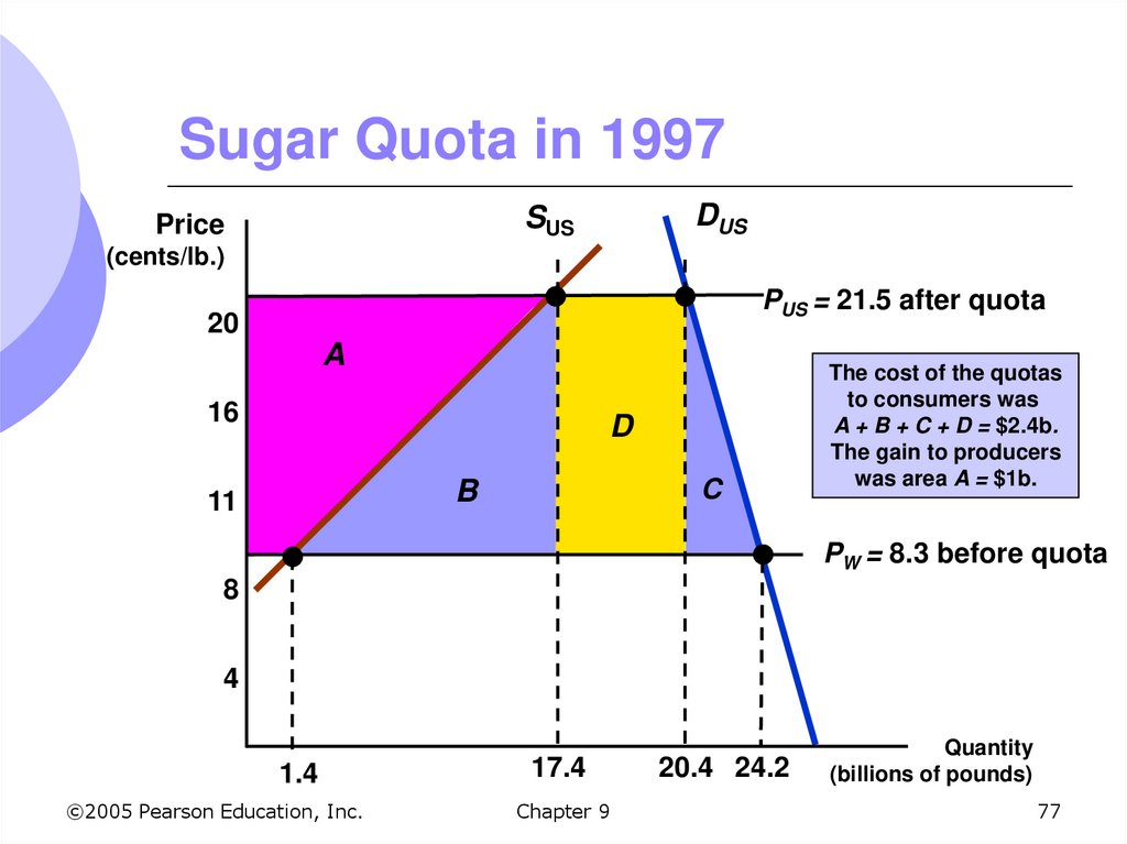
DUS
SUS
Price
(cents/lb.)
PUS = 21.5 after quota
20
A
16
D
C
B
11
The cost of the quotas
to consumers was
A + B + C + D = $2.4b.
The gain to producers
was area A = $1b.
PW = 8.3 before quota
8
4
1.4
©2005 Pearson Education, Inc.
17.4
Chapter 9
20.4 24.2
Quantity
(billions of pounds)
77

78. The Impact of a Tax or Subsidy

The government wants to impose a $1.00
tax on movies. It can do it two ways:
Make the producers pay $1.00 for each
movie ticket they sell
Make consumers pay $1.00 when they buy
each movie
In which option are consumers paying
more?
©2005 Pearson Education, Inc.
Chapter 9
78

79. The Impact of a Tax or Subsidy

The burden of a tax (or the benefit of a
subsidy) falls partly on the consumer and
partly on the producer
How the burden is split between the
parties depends on the relative
elasticities of demand and supply
©2005 Pearson Education, Inc.
Chapter 9
79

80. The Effects of a Specific Tax

For simplicity we will consider a specific
tax on a good
Tax of a particular amount per unit sold
Federal and state taxes on gas and
cigarettes
For our example, consider a specific tax
of $t per widget sold
©2005 Pearson Education, Inc.
Chapter 9
80

81. Incidence of a Specific Tax

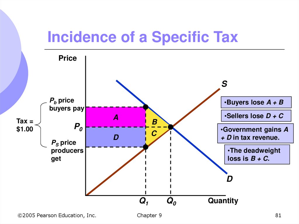
Price
S
Pb price
buyers pay
Tax =
$1.00
•Buyers lose A + B
A
B
P0
PS price
producers
get
•Sellers lose D + C
•Government gains A
+ D in tax revenue.
C
D
•The deadweight
loss is B + C.
D
Q1
©2005 Pearson Education, Inc.
Chapter 9
Q0
Quantity
81

82. Incidence of a Specific Tax

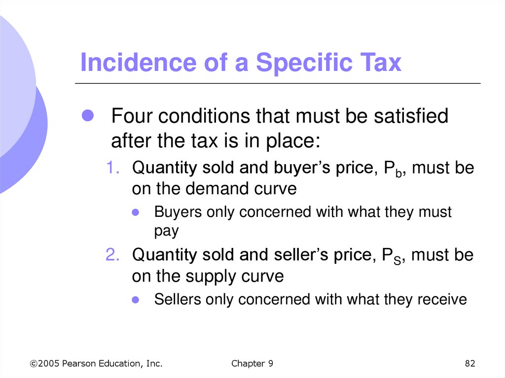
Four conditions that must be satisfied
after the tax is in place:
1. Quantity sold and buyer’s price, Pb, must be
on the demand curve
Buyers only concerned with what they must
pay
2. Quantity sold and seller’s price, PS, must be
on the supply curve
Sellers only concerned with what they receive
©2005 Pearson Education, Inc.
Chapter 9
82

83. Incidence of a Specific Tax

Four conditions that must be satisfied
after the tax is in place (cont.):
3. QD = QS
4. Difference between what consumers pay
and what buyers receive is the tax
If we know the demand and supply
curves as well as the tax, we can solve
for PB, PS, QD and QS
©2005 Pearson Education, Inc.
Chapter 9
83

84. Incidence of a Specific Tax

In the previous example, the tax was
shared almost equally by consumers and
producers
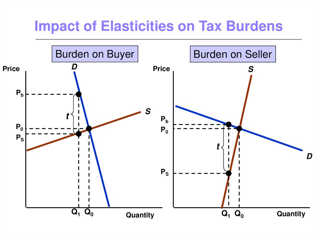
If demand is relatively inelastic, however,
burden of tax will fall mostly on buyers
Cigarettes
If supply is relatively inelastic, the burden
of tax will fall mostly on sellers
©2005 Pearson Education, Inc.
Chapter 9
84

85. Impact of Elasticities on Tax Burdens

Burden on Buyer
Burden on Seller
D
Price
Price
S
Pb
S
t
Pb
P0
P0
PS
t
D
PS
Q1 Q 0
Quantity
Q1 Q0
Quantity

86. The Impact of a Tax or Subsidy

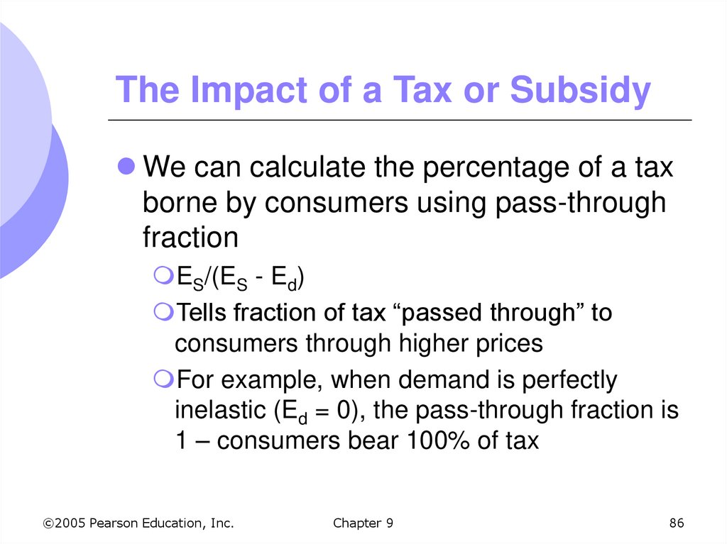
We can calculate the percentage of a tax
borne by consumers using pass-through
fraction
ES/(ES - Ed)
Tells fraction of tax “passed through” to
consumers through higher prices
For example, when demand is perfectly
inelastic (Ed = 0), the pass-through fraction is
1 – consumers bear 100% of tax
©2005 Pearson Education, Inc.
Chapter 9
86

87. The Effects of a Tax or Subsidy

A subsidy can be analyzed in much the
same way as a tax
Payment reducing the buyer’s price below
the seller’s price
It can be treated as a negative tax
The seller’s price exceeds the buyer’s
price
Quantity increases
©2005 Pearson Education, Inc.
Chapter 9
87

88. Effects of a Subsidy

Price
S
Like a tax, the benefit
of a subsidy is split
between buyers and
sellers, depending
upon the elasticities of
supply and demand.
PS
Subsidy
P0
Pb
D
Q0
©2005 Pearson Education, Inc.
Chapter 9
Q1
Quantity
88

89. Effects of a Subsidy

The benefit of the subsidy accrues mostly
to buyers if ED /ES is small
The benefit of the subsidy accrues mostly
to sellers if ES /ES is large
As with a tax, using supply and demand
curves, and the size of the subsidy, one
can solve for resulting prices and
quantities
©2005 Pearson Education, Inc.
Chapter 9
89

90. A Tax on Gasoline

We can measure the effects of a tax by
looking at an example of a gasoline tax
The goal of a large gasoline tax is to:
Raise government revenue
Reduce oil consumption and reduce US
dependence on oil imports
We will consider a gas tax in the market
during mid-1990’s
©2005 Pearson Education, Inc.
Chapter 9
90

91. A Tax on Gasoline

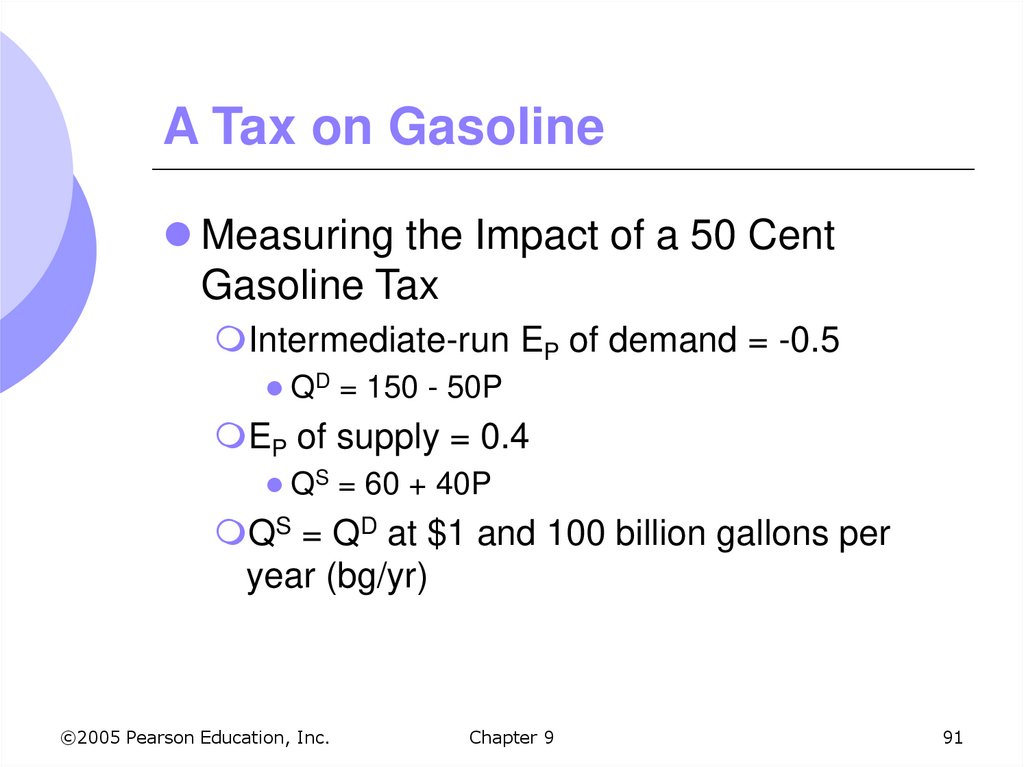
Measuring the Impact of a 50 Cent
Gasoline Tax
Intermediate-run EP of demand = -0.5
QD = 150 - 50P
EP of supply = 0.4
QS = 60 + 40P
QS = QD at $1 and 100 billion gallons per
year (bg/yr)
©2005 Pearson Education, Inc.
Chapter 9
91

92. A Tax on Gasoline

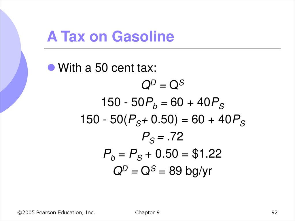
With a 50 cent tax:
QD = QS
150 - 50Pb = 60 + 40PS
150 - 50(PS+ 0.50) = 60 + 40PS
PS = .72
Pb = PS + 0.50 = $1.22
QD = QS = 89 bg/yr
©2005 Pearson Education, Inc.
Chapter 9
92

93. A Tax on Gasoline

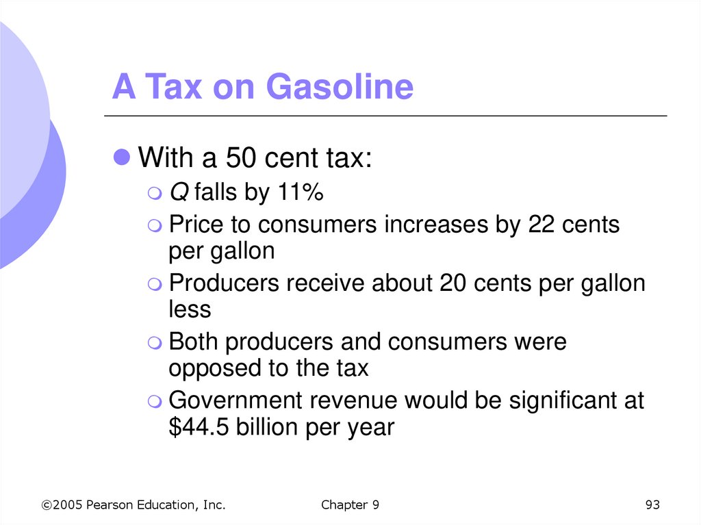
With a 50 cent tax:
Q falls by 11%
Price to consumers increases by 22 cents
per gallon
Producers receive about 20 cents per gallon
less
Both producers and consumers were
opposed to the tax
Government revenue would be significant at
$44.5 billion per year
©2005 Pearson Education, Inc.
Chapter 9
93

94. The Impact of a 50 Cent Gasoline Tax

D
Price
($ per
gallon)
S
Consumer Loss = A + B
B
Producer Loss = C + D
Pb = 1.22
A
$0.50
Tax
P0 = 1.00
C
D
PS = .72
The buyer pays 22 cents of
the tax, and
the producer pays 28 cents.
Government revenue = A + D
= 0.50(89) = $44.5 billion.
11
50 60
©2005 Pearson Education, Inc.
89 100
Chapter 9
150
Quantity (billion
gallons per year)
94