Pricing with Market Power. Chapter 11

1. Chapter 11

Pricing with Market Power

2. Topics to be Discussed

Capturing Consumer Surplus
Price Discrimination
Intertemporal Price Discrimination and
Peak-Load Pricing
The Two-Part Tariff
Bundling
Advertising
©2005 Pearson Education, Inc.
Chapter 11
2

3. Introduction

Pricing without market power (perfect
competition) is determined by market
supply and demand
The individual producer must be able to
forecast the market and then concentrate
on managing production (cost) to
maximize profits
©2005 Pearson Education, Inc.
Chapter 11
3

4. Introduction

Pricing with market power (imperfect
competition) requires the individual
producer to know much more about the
characteristics of demand as well as
manage production
©2005 Pearson Education, Inc.
Chapter 11
4

5. Capturing Consumer Surplus

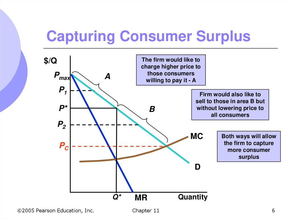
All pricing strategies we will examine are
means of capturing consumer surplus
and transferring it to the producer
Profit maximizing point of P* and Q*
But some consumers will pay more than P*
for a good
Raising price will lose some consumers, leading
to smaller profits
Lowering price will gain some consumers, but
lower profits
©2005 Pearson Education, Inc.
Chapter 11
5

6. Capturing Consumer Surplus

$/Q
Pmax
The firm would like to
charge higher price to
those consumers
willing to pay it - A
A
P1
P*
B
Firm would also like to
sell to those in area B but
without lowering price to
all consumers
P2
MC
PC
Both ways will allow
the firm to capture
more consumer
surplus
D
Q*
©2005 Pearson Education, Inc.
MR
Chapter 11
Quantity
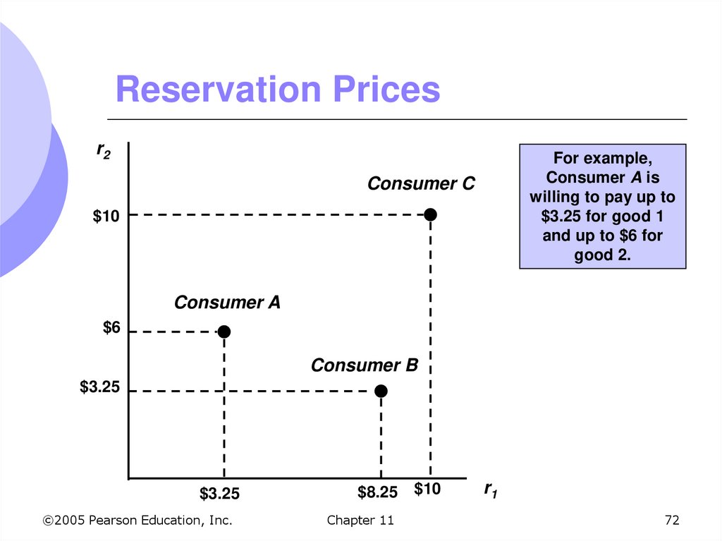
6

7. Capturing Consumer Surplus

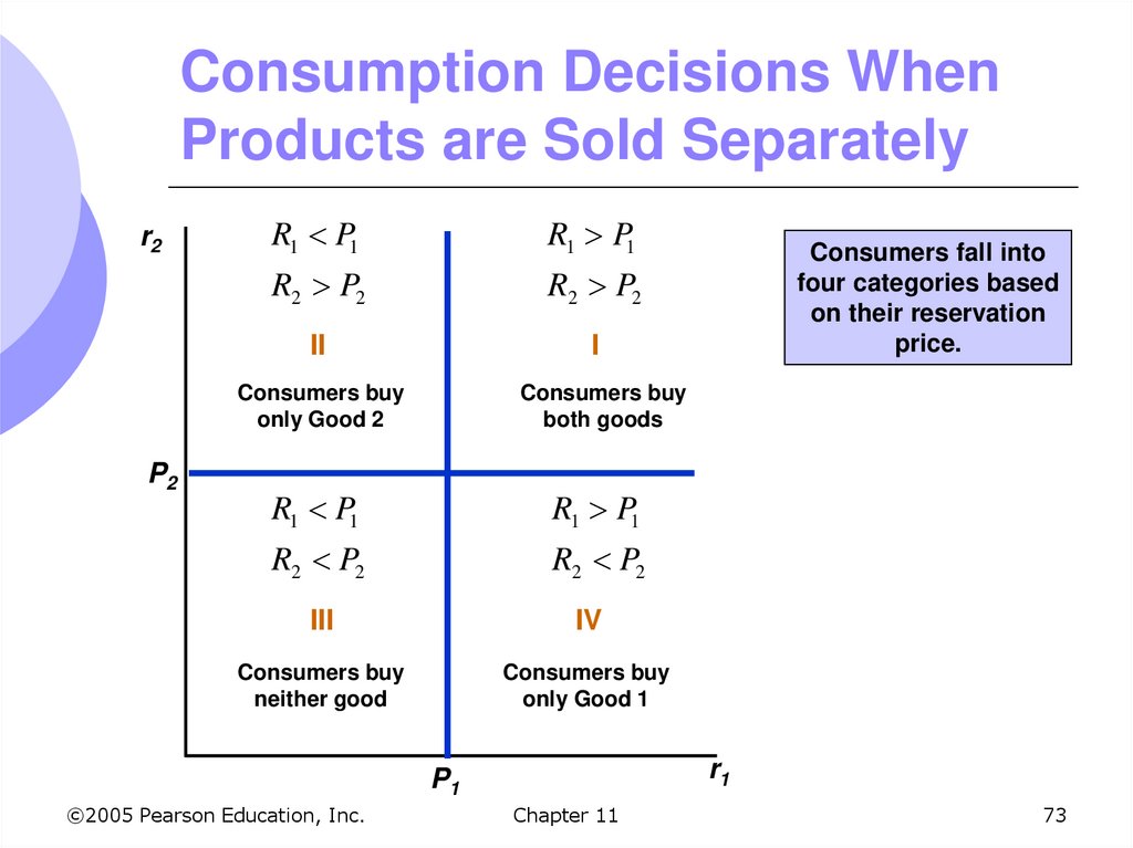
Price discrimination is the practice of
charging different prices to different
consumers for similar goods
Must be able to identify the different
consumers and get them to pay different
prices
Other techniques that expand the range
of a firm’s market to get at more
consumer surplus
Tariffs and bundling
©2005 Pearson Education, Inc.
Chapter 11
7

8. Price Discrimination

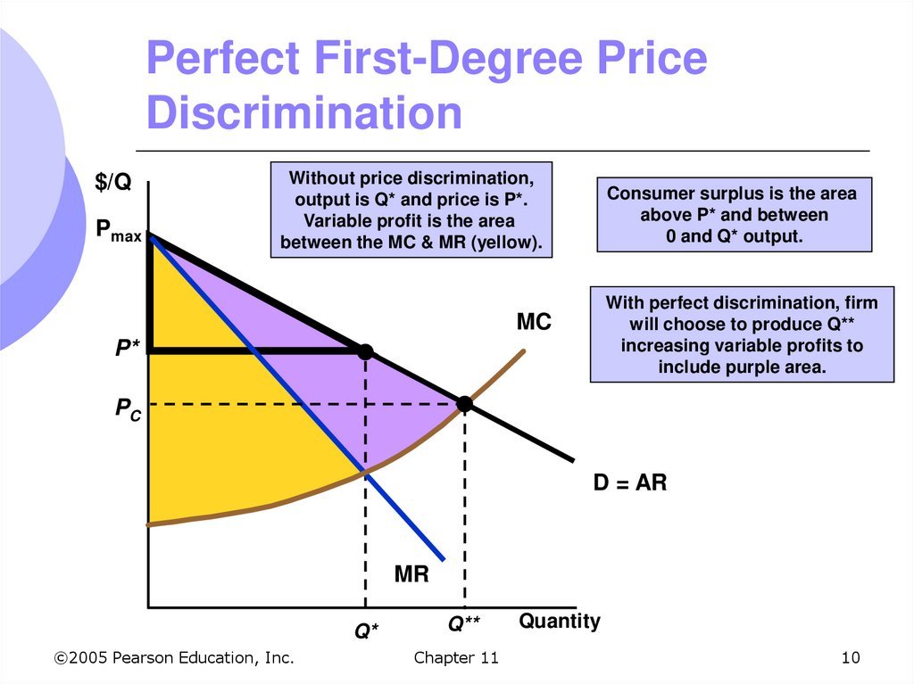
First Degree Price Discrimination
Charge a separate price to each customer: the
maximum or reservation price they are willing to pay
How can a firm profit?
The firm produces Q* MR = MC
We can see the firm’s variable profit – the firm’s profit
ignoring fixed costs
Area between MR and MC
Consumer surplus area between demand and price
©2005 Pearson Education, Inc.
Chapter 11
8

9. Price Discrimination

If the firm can price discriminate perfectly,
each consumer is charged exactly what
they are willing to pay
MR curve is no longer part of output decision
Incremental revenue is exactly the price at
which each unit is sold – the demand curve
Additional profit from producing and selling
an incremental unit is now the difference
between demand and marginal cost
©2005 Pearson Education, Inc.
Chapter 11
9

10. Perfect First-Degree Price Discrimination

$/Q
Pmax
Without price discrimination,
output is Q* and price is P*.
Variable profit is the area
between the MC & MR (yellow).
Consumer surplus is the area
above P* and between
0 and Q* output.
With perfect discrimination, firm
will choose to produce Q**
increasing variable profits to
include purple area.
MC
P*
PC
D = AR
MR
Q*
©2005 Pearson Education, Inc.
Q**
Chapter 11
Quantity
10

11. First-Degree Price Discrimination

In practice, perfect price discrimination
is almost never possible
1. Impractical to charge every customer a
different price (unless very few customers)
2. Firms usually do not know reservation price
of each customer
Firms can discriminate imperfectly
Can charge a few different prices based on
some estimates of reservation prices
©2005 Pearson Education, Inc.
Chapter 11
11

12. First-Degree Price Discrimination

Examples of imperfect price
discrimination where the seller has the
ability to segregate the market to some
extent and charge different prices for the
same product:
Lawyers, doctors, accountants
Car salesperson (15% profit margin)
Colleges and universities (differences in
financial aid)
©2005 Pearson Education, Inc.
Chapter 11
12

13. First-Degree Price Discrimination in Practice

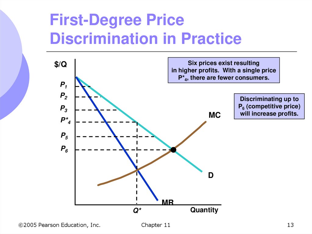
Six prices exist resulting
in higher profits. With a single price
P*4, there are fewer consumers.
$/Q
P1
P2
P3
MC
P*4
Discriminating up to
P6 (competitive price)
will increase profits.
P5
P6
D
MR
Quantity
Q*
©2005 Pearson Education, Inc.
Chapter 11
13

14. Second-Degree Price Discrimination

In some markets, consumers purchase
many units of a good over time
Demand for that good declines with
increased consumption
Electricity, water, heating fuel
Firms can engage in second-degree price
discrimination
Practice of charging different prices per unit for
different quantities of the same good or service
©2005 Pearson Education, Inc.
Chapter 11
14

15. Second-Degree Price Discrimination

Quantity discounts are an example of
second-degree price discrimination
Ex: Buying in bulk at Sam’s Club
Block pricing – the practice of charging
different prices for different quantities of
“blocks” of a good
Ex: electric power companies charge
different prices for a consumer purchasing a
set block of electricity
©2005 Pearson Education, Inc.
Chapter 11
15

16. Second-Degree Price Discrimination

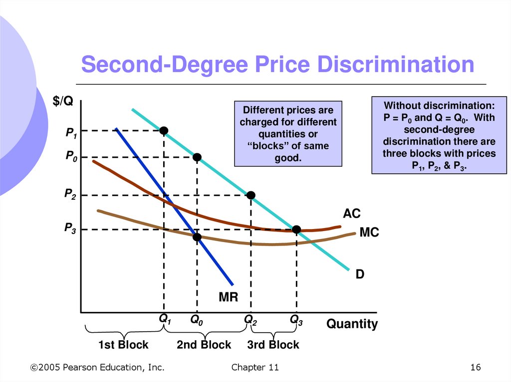
$/Q
Without discrimination:
P = P0 and Q = Q0. With
second-degree
discrimination there are
three blocks with prices
P1, P2, & P3.
Different prices are
charged for different
quantities or
“blocks” of same
good.
P1
P0
P2
AC
MC
P3
D
MR
Q1
1st Block
©2005 Pearson Education, Inc.
Q0
2nd Block
Q2
Q3
Quantity
3rd Block
Chapter 11
16

17. Third-Degree Price Discrimination

Practice of dividing consumers into two
or more groups with separate demand
curves and charging different prices to
each group
1. Divides the market into two groups
2. Each group has its own demand function
©2005 Pearson Education, Inc.
Chapter 11
17

18. Price Discrimination

Third Degree Price Discrimination
Most common type of price discrimination
Examples: airlines, premium vs. nonpremium liquor, discounts to students and
senior citizens, frozen vs. canned vegetables
©2005 Pearson Education, Inc.
Chapter 11
18

19. Third-Degree Price Discrimination

Same characteristic is used to divide the
consumer groups
Typically, elasticities of demand differ for
the groups
College students and senior citizens are not
usually willing to pay as much as others
because of lower incomes
These groups are easily distinguishable with
ID’s
©2005 Pearson Education, Inc.
Chapter 11
19

20. Creating Consumer Groups

If third-degree price discrimination is
feasible, how can the firm decide what
to charge each group of consumers?
1. Total output should be divided between
groups so that MR for each group is equal
2. Total output is chosen so that MR for each
group of consumers is equal to the MC of
production
©2005 Pearson Education, Inc.
Chapter 11
20

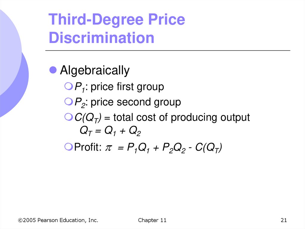
21. Third-Degree Price Discrimination

Algebraically
P1: price first group
P2: price second group
C(QT) = total cost of producing output
QT = Q 1 + Q 2
Profit: = P1Q1 + P2Q2 - C(QT)
©2005 Pearson Education, Inc.
Chapter 11
21

22. Third-Degree Price Discrimination

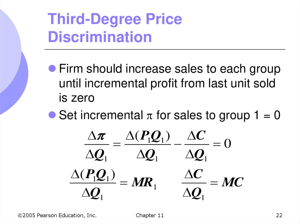
Firm should increase sales to each group
until incremental profit from last unit sold
is zero
Set incremental for sales to group 1 = 0
( P1Q1 ) C
0
Q1
Q1
Q1
( P1Q1 )
MR1
Q1
©2005 Pearson Education, Inc.
Chapter 11
C
MC
Q1
22

23. Third-Degree Price Discrimination

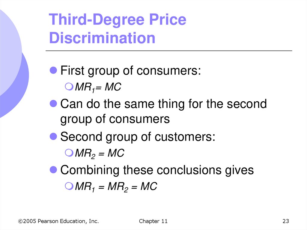
First group of consumers:
MR1= MC
Can do the same thing for the second
group of consumers
Second group of customers:
MR2 = MC
Combining these conclusions gives
MR1 = MR2 = MC
©2005 Pearson Education, Inc.
Chapter 11
23

24. Third-Degree Price Discrimination

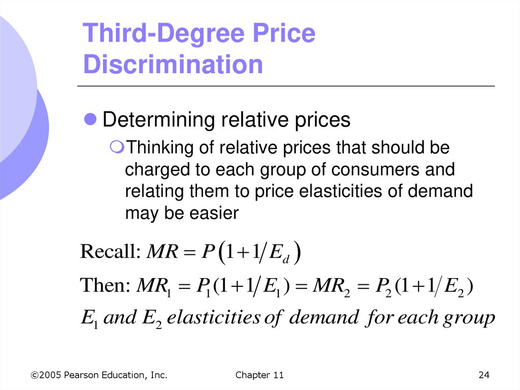
Determining relative prices
Thinking of relative prices that should be
charged to each group of consumers and
relating them to price elasticities of demand
may be easier
Recall: MR P 1 1 Ed
Then: MR1 P1 (1 1 E1 ) MR2 P2 (1 1 E2 )
E1 and E2 elasticities of demand for each group
©2005 Pearson Education, Inc.
Chapter 11
24

25. Third-Degree Price Discrimination

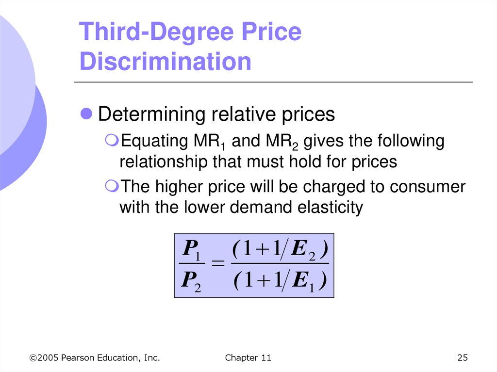
Determining relative prices
Equating MR1 and MR2 gives the following
relationship that must hold for prices
The higher price will be charged to consumer
with the lower demand elasticity
P1 ( 1 1 E 2 )
P2 ( 1 1 E1 )
©2005 Pearson Education, Inc.
Chapter 11
25

26. Third-Degree Price Discrimination

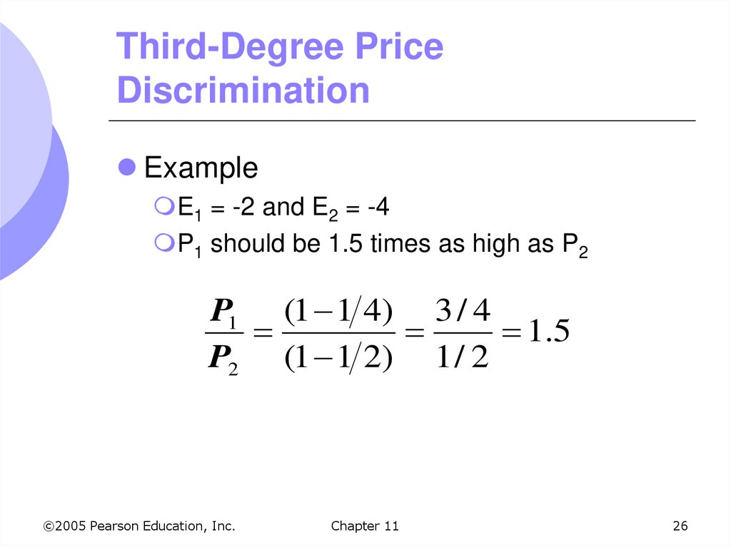
Example
E1 = -2 and E2 = -4
P1 should be 1.5 times as high as P2
P1 (1 1 4) 3 / 4
1.5
P2 (1 1 2) 1 / 2
©2005 Pearson Education, Inc.
Chapter 11
26

27. Third-Degree Price Discrimination

$/Q
Consumers are divided into
two groups, with separate
demand curves for each group.
MRT = MR1 + MR2
D2 = AR2
MRT
MR2
MR1
©2005 Pearson Education, Inc.
D1 = AR1
Chapter 11
Quantity
27

28. Third-Degree Price Discrimination

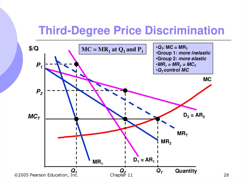
$/Q
MC = MR1 at Q1 and P1
P1
•QT: MC = MRT
•Group 1: more inelastic
•Group 2: more elastic
•MR1 = MR2 = MCT
•QT control MC
MC
P2
D2 = AR2
MCT
MRT
MR2
D1 = AR1
MR1
Q1
©2005 Pearson Education, Inc.
Q2
Chapter 11
QT
Quantity
28

29. No Sales to Smaller Market

Even if third-degree price discrimination
is possible, it may not be feasible to try to
sell to both groups
It is possible that the demand for one group
is so low that it would not be profitable to
lower price enough to sell to that group
©2005 Pearson Education, Inc.
Chapter 11
29

30. No Sales to Smaller Market

Group one, with
demand D1, is not
willing to pay enough
for the good to make
price discrimination
profitable.
$/Q
MC
P*
D2
MC=MR1
=MR2
MR2
MR1
D1
Q*
©2005 Pearson Education, Inc.
Chapter 11
Quantity
30

31. The Economics of Coupons and Rebates

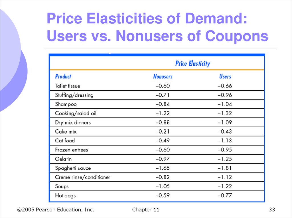
Those consumers who are more price
elastic will tend to use the coupon/rebate
more often when they purchase the
product than those consumers with a less
elastic demand
Coupons and rebate programs allow
firms to price discriminate
©2005 Pearson Education, Inc.
Chapter 11
31

32. The Economics of Coupons and Rebates

About 20 – 30% of consumers use
coupons or rebates
Firms can get those with higher
elasticities of demand to purchase the
good who would not normally buy it
Table 11.1 shows how elasticities of
demand vary for coupon/rebate users
and non-users
©2005 Pearson Education, Inc.
Chapter 11
32

33. Price Elasticities of Demand: Users vs. Nonusers of Coupons

©2005 Pearson Education, Inc.
Chapter 11
33

34. Airline Fares

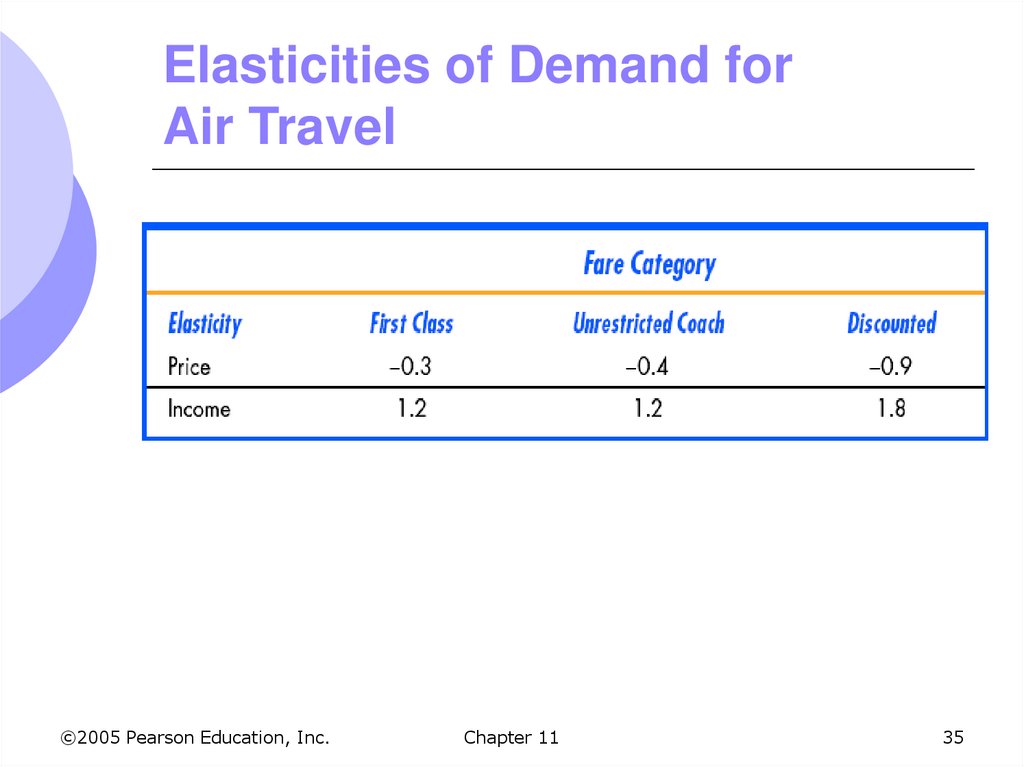
Differences in elasticities imply that some
customers will pay a higher fare than
others
Business travelers have few choices and
their demand is less elastic
Casual travelers and families are more
price-sensitive and will therefore be
choosier
©2005 Pearson Education, Inc.
Chapter 11
34

35. Elasticities of Demand for Air Travel

©2005 Pearson Education, Inc.
Chapter 11
35

36. Airline Fares

There are multiple fares for every route
flown by airlines
They separate the market by setting
various restrictions on the tickets
Must stay over a Saturday night
21-day advance, 14-day advance
Basic restrictions – can change ticket to only
certain days
Most expensive: no restrictions – first class
©2005 Pearson Education, Inc.
Chapter 11
36

37. Other Types of Price Discrimination

Intertemporal Price Discrimination
Practice of separating consumers with
different demand functions into different
groups by charging different prices at
different points in time
Initial release of a product, the demand is
inelastic
Hard back vs. paperback book
New release movie
Technology
©2005 Pearson Education, Inc.
Chapter 11
37

38. Intertemporal Price Discrimination

Once this market has yielded a maximum
profit, firms lower the price to appeal to a
general market with a more elastic
demand
This can be seen graphically looking at
two different groups of consumers – one
willing to buy right now and one willing to
wait
©2005 Pearson Education, Inc.
Chapter 11
38

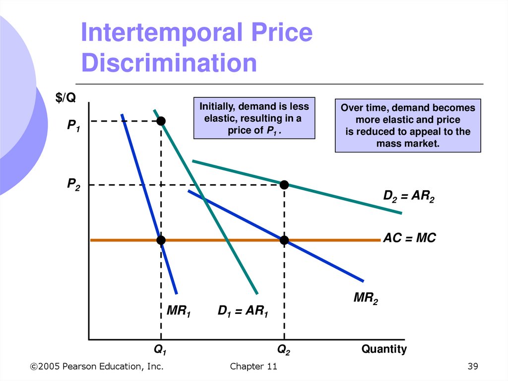
39. Intertemporal Price Discrimination

$/Q
Initially, demand is less
elastic, resulting in a
price of P1 .
P1
Over time, demand becomes
more elastic and price
is reduced to appeal to the
mass market.
P2
D2 = AR2
AC = MC
MR1
Q1
©2005 Pearson Education, Inc.
MR2
D1 = AR1
Q2
Chapter 11
Quantity
39

40. Other Types of Price Discrimination

Peak-Load Pricing
Practice of charging higher prices during
peak periods when capacity constraints
cause marginal costs to be higher
Demand for some products may peak at
particular times
Rush hour traffic
Electricity - late summer afternoons
Ski resorts on weekends
©2005 Pearson Education, Inc.
Chapter 11
40

41. Peak-Load Pricing

Objective is to increase efficiency by
charging customers close to marginal
cost
Increased MR and MC would indicate a
higher price
Total surplus is higher because charging
close to MC
Can measure efficiency gain from peak-load
pricing
©2005 Pearson Education, Inc.
Chapter 11
41

42. Peak-Load Pricing

With third-degree price discrimination,
the MR for all markets was equal
MR is not equal for each market because
one market does not impact the other
market with peak-load pricing
Price and sales in each market are
independent
Ex: electricity, movie theaters
©2005 Pearson Education, Inc.
Chapter 11
42

43. Peak-Load Pricing

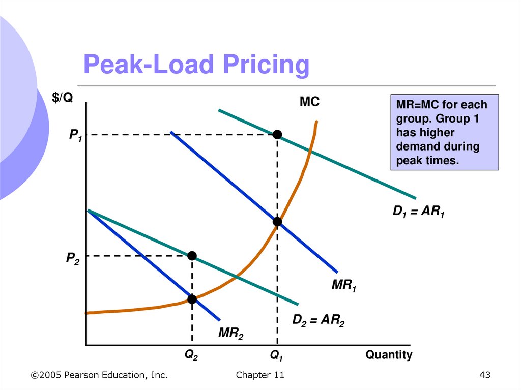
$/Q
MC
MR=MC for each
group. Group 1
has higher
demand during
peak times.
P1
D1 = AR1
P2
MR1
D2 = AR2
MR2
Q2
©2005 Pearson Education, Inc.
Q1
Chapter 11
Quantity
43

44. How to Price a Best-Selling Novel

How would you arrive at the price for the
initial release of the hardbound edition of
a book?
Hardback and paperback books are ways for
the company to price discriminate
How does the company determine what price
to sell the hardback and paperback books
for?
How does the company determine when to
release the paperback?
©2005 Pearson Education, Inc.
Chapter 11
44

45. How to Price a Best-Selling Novel

Company must divide consumers into
two groups:
Those willing to buy the more expensive
hardback
Those willing to wait for the paperback
Have to be strategic about when to
release paperback after hardback
Publishers typically wait 12 to 18 months
©2005 Pearson Education, Inc.
Chapter 11
45

46. How to Price a Best-Selling Novel

Publishers must use estimates of past
books to determine how much to sell a
new book for
Hard to determine the demand for a
NEW book
New books are typically sold for about
the same price, to take this into account
Demand for paperbacks is more elastic
so we should expect it to be priced lower
©2005 Pearson Education, Inc.
Chapter 11
46

47. The Two-Part Tariff

Form of pricing in which consumers are charged
both an entry and usage fee
Ex: amusement park, golf course, telephone service
A fee is charged upfront for right to use/buy the
product
An additional fee is charged for each unit the
consumer wishes to consume
Pay a fee to play golf and then pay another fee for
each game you play
©2005 Pearson Education, Inc.
Chapter 11
47

48. The Two-Part Tariff

Pricing decision is setting the entry fee
(T) and the usage fee (P)
Choosing the trade-off between freeentry and high-use prices or high-entry
and zero-use prices
Single Consumer
Assume firm knows consumer demand
Firm wants to capture as much consumer
surplus as possible
©2005 Pearson Education, Inc.
Chapter 11
48

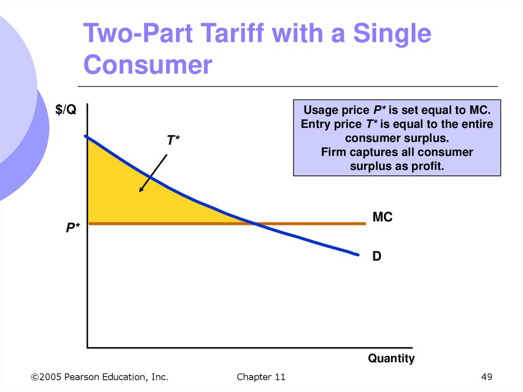
49. Two-Part Tariff with a Single Consumer

$/Q
Usage price P* is set equal to MC.
Entry price T* is equal to the entire
consumer surplus.
Firm captures all consumer
surplus as profit.
T*
MC
P*
D
Quantity
©2005 Pearson Education, Inc.
Chapter 11
49

50. Two-Part Tariff with Two Consumers

Two consumers, but firm can only set one entry
fee and one usage fee
Will no longer set usage fee equal to MC
Could make entry fee no larger than CS of consumer
with smallest demand
Firm should set usage fee above MC
Set entry fee equal to remaining consumer
surplus of consumer with smaller demand
Firm needs to know demand curves
©2005 Pearson Education, Inc.
Chapter 11
50

51. Two-Part Tariff with Two Consumers

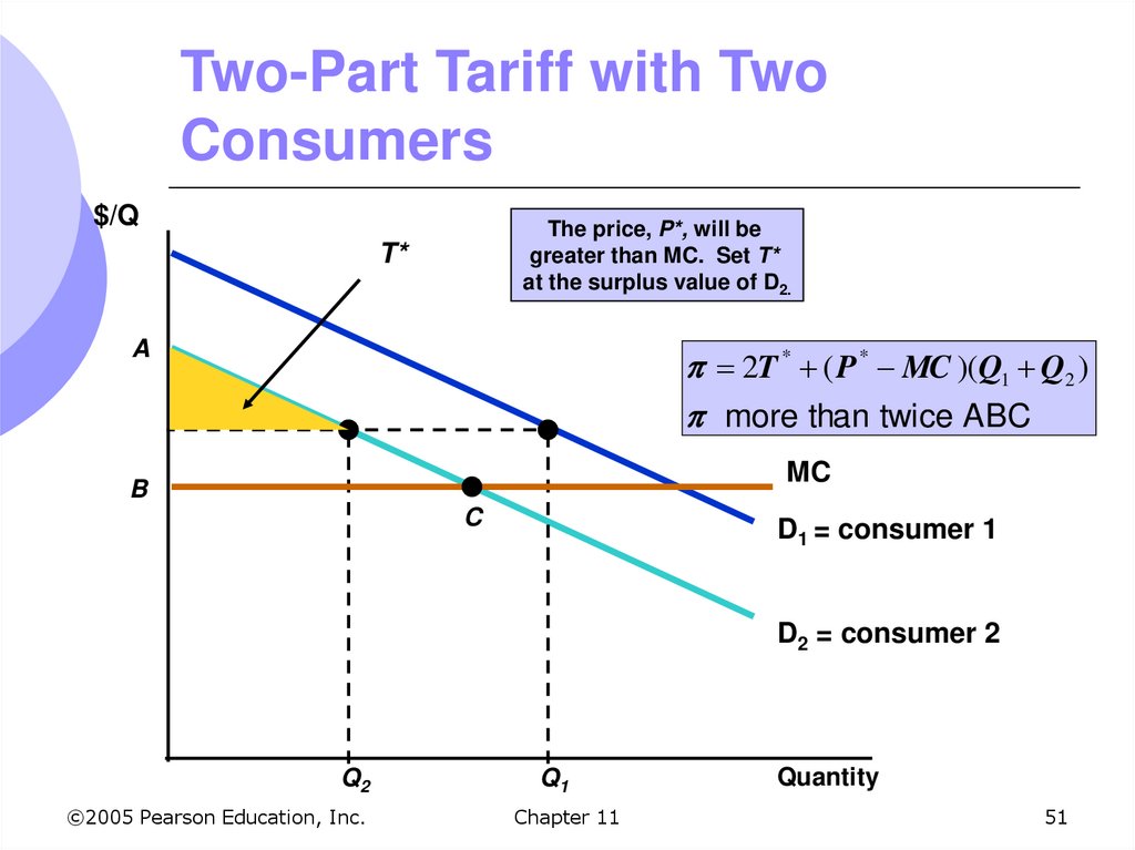
$/Q
The price, P*, will be
greater than MC. Set T*
at the surplus value of D2.
T*
A
2T * ( P * MC )(Q1 Q2 )
more than twice ABC
MC
B
C
D1 = consumer 1
D2 = consumer 2
Q2
©2005 Pearson Education, Inc.
Q1
Chapter 11
Quantity
51

52. The Two-Part Tariff with Many Consumers

No exact way to determine P* and T*
Must consider the trade-off between the
entry fee T* and the use fee P*
Low entry fee: more entrants and more profit
from sales of item
As entry fee becomes smaller, number of
entrants is larger and profit from entry fee will
fall
©2005 Pearson Education, Inc.
Chapter 11
52

53. The Two-Part Tariff with Many Consumers

To find optimum combination, choose
several combinations of P and T
Find combination that maximizes profit
Firm’s profit is divided into two
components
Each is a function of entry fee, T assuming a
fixed sales price, P
©2005 Pearson Education, Inc.
Chapter 11
53

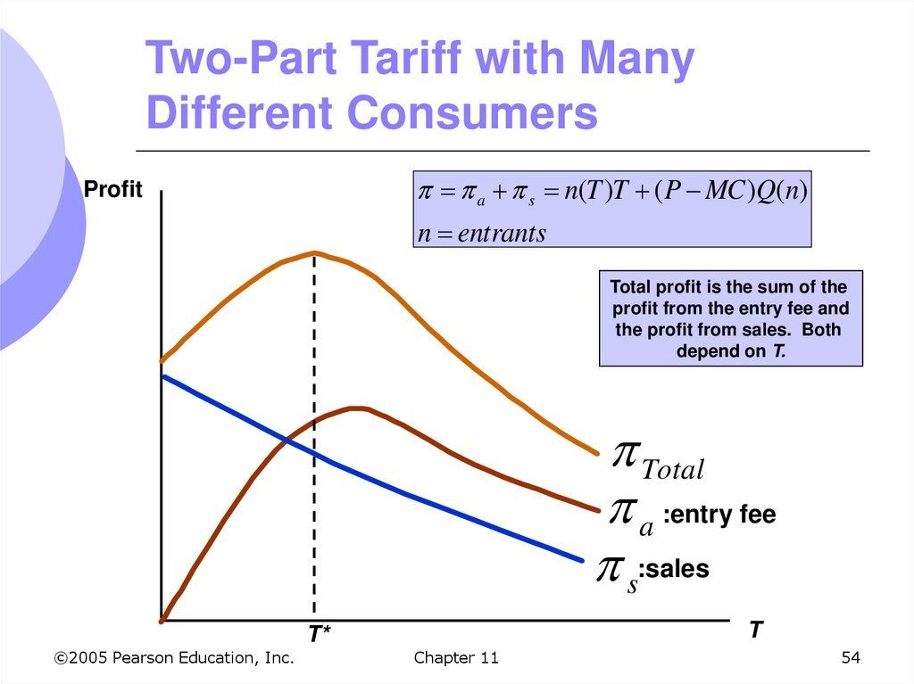
54. Two-Part Tariff with Many Different Consumers

a s n(T )T ( P MC )Q(n)
n entrants
Profit
Total profit is the sum of the
profit from the entry fee and
the profit from sales. Both
depend on T.
Total
a :entry fee
s:sales
T
T*
©2005 Pearson Education, Inc.
Chapter 11
54

55. The Two-Part Tariff

Rule of Thumb
Similar demand: Choose P close to MC and
high T
Dissimilar demand: Choose high P and low T
Ex: Disneyland in California and Disney
world in Florida have a strategy of high entry
fee and charge nothing for ride
©2005 Pearson Education, Inc.
Chapter 11
55

56. The Two-Part Tariff With a Twist

Entry price (T) entitles the buyer to a certain
number of free units
Gillette razors sold with several blades
Amusement park admission comes with some tokens
On-line fees with free time
Can set higher entry fee without losing many
consumers
Higher entry fee captures either surplus without
driving them out of the market
Captures more surplus of large customers
©2005 Pearson Education, Inc.
Chapter 11
56

57. Polaroid Cameras

In 1971, Polaroid introduced the SX-70
camera
Polaroid was able to use two-part tariff for
pricing of camera/film
Allowed them greater profits than would have
been possible if camera used ordinary film
Polaroid had a monopoly on cameras
and film
©2005 Pearson Education, Inc.
Chapter 11
57

58. Polaroid Cameras

Buying camera is like entry fee
Unlike an amusement park, for example, the
marginal cost of providing an additional camera
is significantly greater than zero
It was necessary for Polaroid to have monopoly
If ordinary film could be used, the price of film would
be close to MC
Polaroid needed to gain most of its profits from sale of
film
©2005 Pearson Education, Inc.
Chapter 11
58

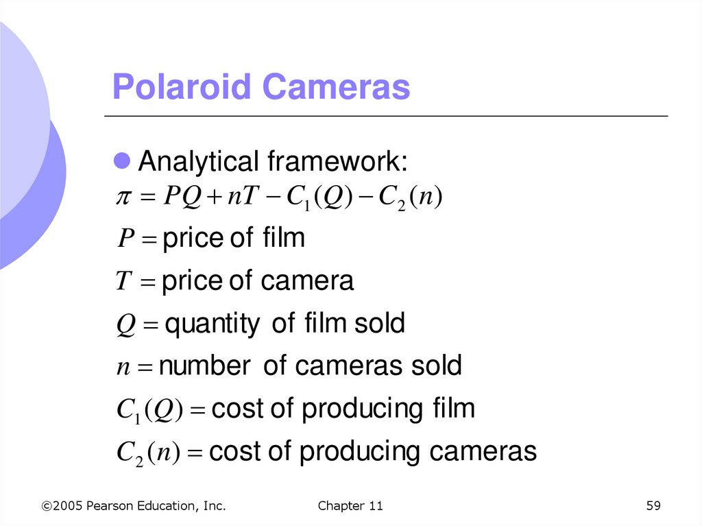
59. Polaroid Cameras

Analytical framework:
PQ nT C1 (Q) C2 (n)
P price of film
T price of camera
Q quantity of film sold
n number of cameras sold
C1 (Q ) cost of producing film
C2 (n) cost of producing cameras
©2005 Pearson Education, Inc.
Chapter 11
59

60. Polaroid Cameras

In the end, the film prices were
significantly above marginal cost
There was considerable heterogeneity of
consumer demands
©2005 Pearson Education, Inc.
Chapter 11
60

61. Cellular Rate Plans

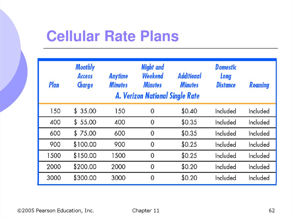
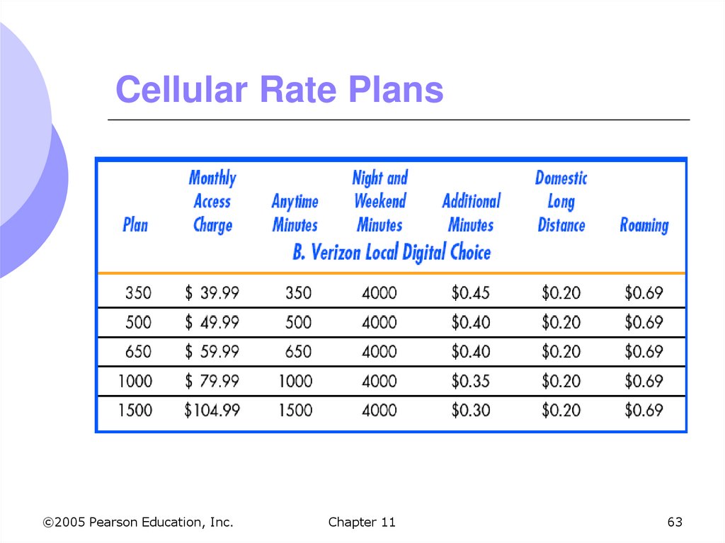
In most areas in US, consumers can choose
cellular providers: Verizon, Cingular, AT&T and
Sprint
Market power exists because consumers face
switching costs
When they sign up with a firm, they must sign a
contract with high costs to break
Plans often exist of monthly cost plus fee extra
minutes
Companies can combine third-degree price
discrimination with two-part tariff
©2005 Pearson Education, Inc.
Chapter 11
61

62. Cellular Rate Plans

©2005 Pearson Education, Inc.
Chapter 11
62

63. Cellular Rate Plans

©2005 Pearson Education, Inc.
Chapter 11
63

64. Bundling

Bundling is packaging two or more
products to gain a pricing advantage
Conditions necessary for bundling
Heterogeneous customers
Price discrimination is not possible
Demands must be negatively correlated
©2005 Pearson Education, Inc.
Chapter 11
64

65. Bundling

When film company leased “Gone with
the Wind,” it required theaters to also
lease “Getting Gertie’s Garter”
Why would a company do this?
Company must be able to increase revenue
We can see the reservation prices for each
theater and movie
©2005 Pearson Education, Inc.
Chapter 11
65

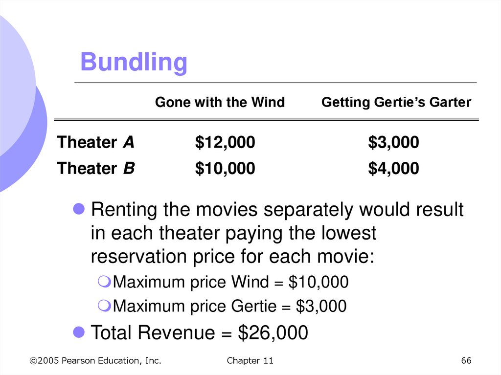
66. Bundling

Gone with the Wind
Getting Gertie’s Garter
Theater A
$12,000
$3,000
Theater B
$10,000
$4,000
Renting the movies separately would result
in each theater paying the lowest
reservation price for each movie:
Maximum price Wind = $10,000
Maximum price Gertie = $3,000
Total Revenue = $26,000
©2005 Pearson Education, Inc.
Chapter 11
66

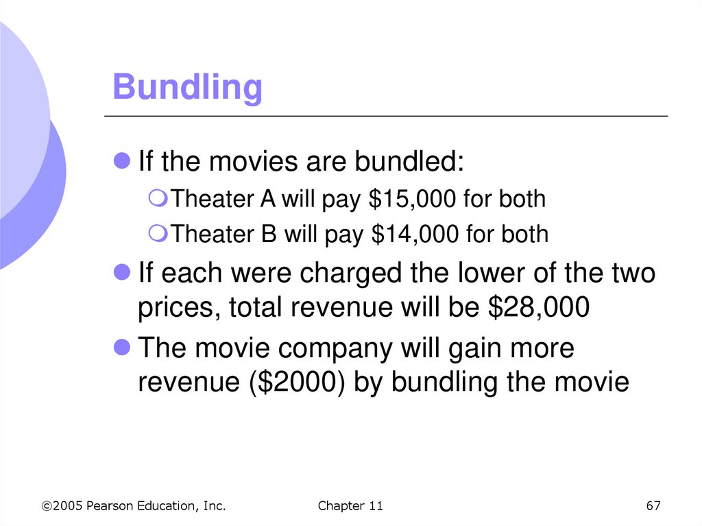
67. Bundling

If the movies are bundled:
Theater A will pay $15,000 for both
Theater B will pay $14,000 for both
If each were charged the lower of the two
prices, total revenue will be $28,000
The movie company will gain more
revenue ($2000) by bundling the movie
©2005 Pearson Education, Inc.
Chapter 11
67

68. Relative Valuations

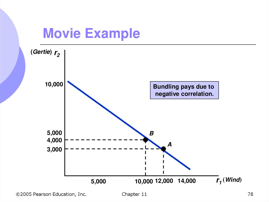
More profitable to bundle because
relative valuation of two films are
reversed
Demands are negatively correlated
A pays more for Wind ($12,000) than B
($10,000)
B pays more for Gertie ($4,000) than A
($3,000)
©2005 Pearson Education, Inc.
Chapter 11
68

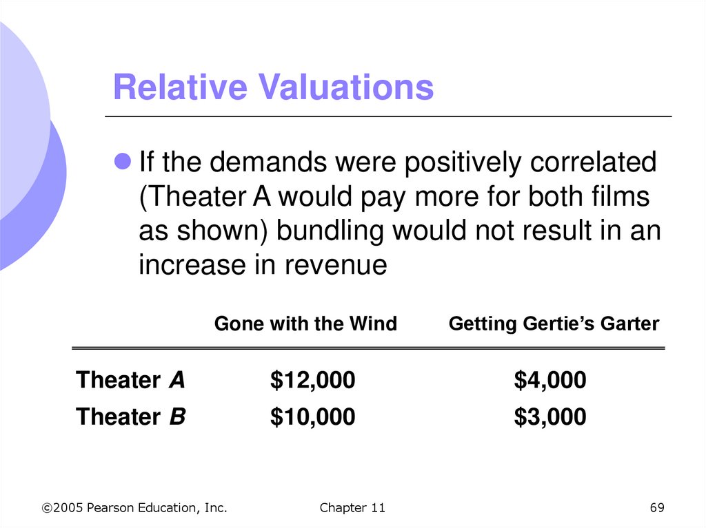
69. Relative Valuations

If the demands were positively correlated
(Theater A would pay more for both films
as shown) bundling would not result in an
increase in revenue
Gone with the Wind
Getting Gertie’s Garter
Theater A
$12,000
$4,000
Theater B
$10,000
$3,000
©2005 Pearson Education, Inc.
Chapter 11
69

70. Bundling

If the movies are bundled:
Theater A will pay $16,000 for both
Theater B will pay $13,000 for both
If each were charged the lower of the two
prices, total revenue will be $26,000, the
same as by selling the films separately
©2005 Pearson Education, Inc.
Chapter 11
70

71. Bundling

Bundling Scenario: Two different goods
and many consumers
Many consumers with different reservation
price combinations for two goods
Can show graphically the preferences of
consumers in terms of reservation prices and
consumption decisions given prices charged
r1 is reservation price of consumer for good 1
r2 is reservation price of consumer for good 2
©2005 Pearson Education, Inc.
Chapter 11
71

72. Reservation Prices

r2
For example,
Consumer A is
willing to pay up to
$3.25 for good 1
and up to $6 for
good 2.
Consumer C
$10
Consumer A
$6
Consumer B
$3.25
$3.25
$8.25
©2005 Pearson Education, Inc.
Chapter 11
$10
r1
72

73. Consumption Decisions When Products are Sold Separately

r2
P2
R1 P1
R1 P1
R2 P2
R2 P2
II
I
Consumers buy
only Good 2
Consumers buy
both goods
R1 P1
R1 P1
R2 P2
R2 P2
III
IV
Consumers buy
neither good
Consumers buy
only Good 1
r1
P1
©2005 Pearson Education, Inc.
Consumers fall into
four categories based
on their reservation
price.
Chapter 11
73

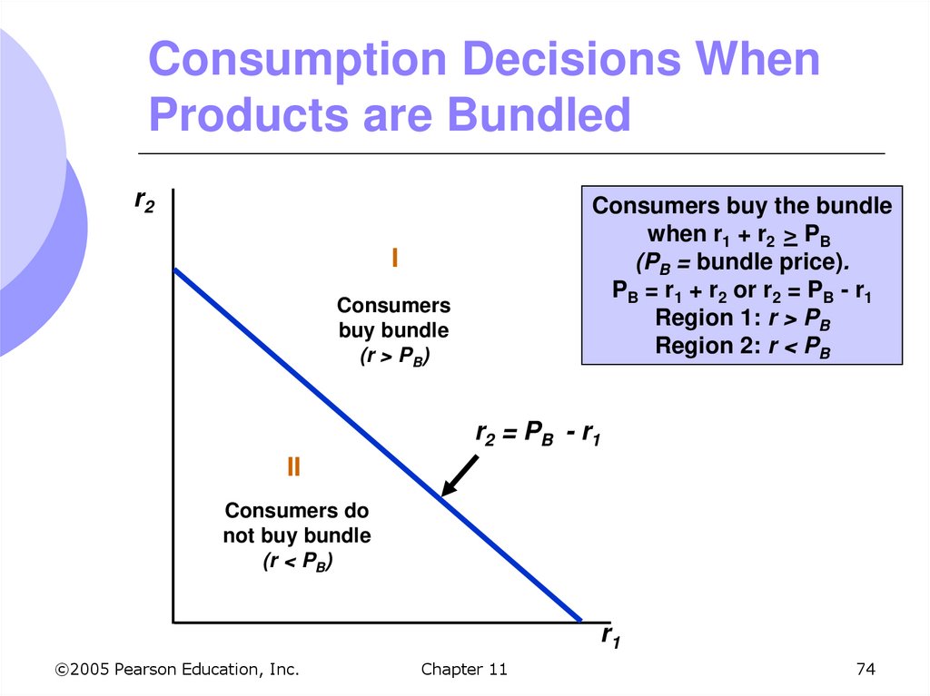
74. Consumption Decisions When Products are Bundled

r2
Consumers buy the bundle
when r1 + r2 > PB
(PB = bundle price).
PB = r1 + r2 or r2 = PB - r1
Region 1: r > PB
Region 2: r < PB
I
Consumers
buy bundle
(r > PB)
r2 = PB - r1
II
Consumers do
not buy bundle
(r < PB)
r1
©2005 Pearson Education, Inc.
Chapter 11
74

75. Consumption Decisions When Products are Bundled

The effectiveness of bundling depends
upon the degree of negative correlation
between the two demands
Best when consumers who have high
reservation price for Good 1 have a low
reservation price for Good 2 and vice versa
Can see graphically looking at positively and
negatively correlated prices
©2005 Pearson Education, Inc.
Chapter 11
75

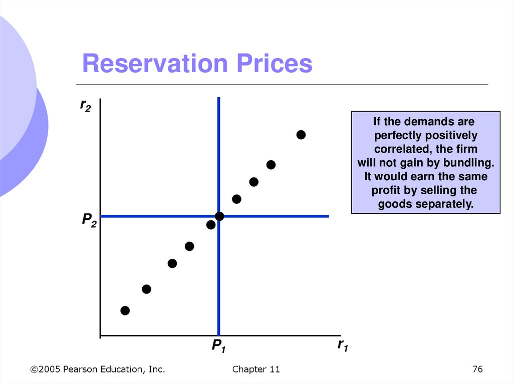
76. Reservation Prices

r2
If the demands are
perfectly positively
correlated, the firm
will not gain by bundling.
It would earn the same
profit by selling the
goods separately.
P2
r1
P1
©2005 Pearson Education, Inc.
Chapter 11
76

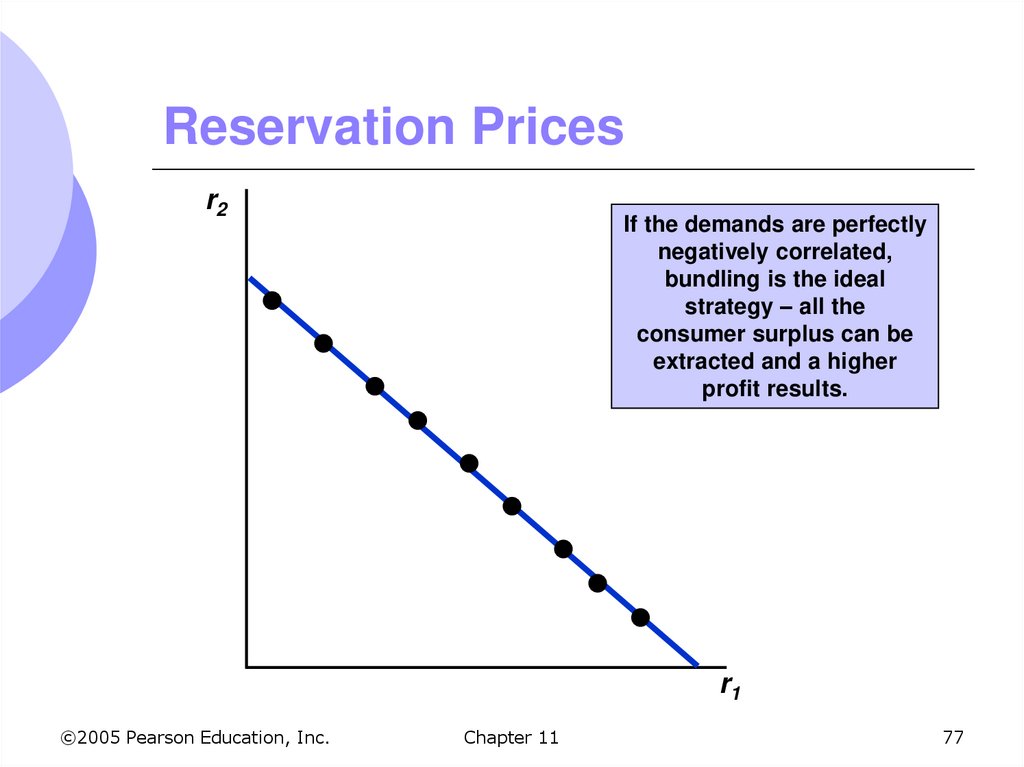
77. Reservation Prices

r2
If the demands are perfectly
negatively correlated,
bundling is the ideal
strategy – all the
consumer surplus can be
extracted and a higher
profit results.
r1
©2005 Pearson Education, Inc.
Chapter 11
77

78. Movie Example

(Gertie) r
2
10,000
Bundling pays due to
negative correlation.
5,000
4,000
B
A
3,000
5,000
©2005 Pearson Education, Inc.
10,000 12,000 14,000
Chapter 11
r1 (Wind)
78

79. Mixed Bundling

Practice of selling two or more goods
both as a package and individually
This differs from pure bundling when
products are sold only as a package
Mixed bundling is good strategy when
Demands are somewhat negatively
correlated
Marginal production costs are significant
©2005 Pearson Education, Inc.
Chapter 11
79

80. Mixed Bundling – Example

Demands are perfectly negatively
correlated but significant marginal costs
Four customers under three different
strategies
Selling good separately, P1 = $50, P2 = $90
Selling goods only as a bundle, PB = $100
Mixed bundling:
Sold individually with P1 = P2 = $89.95
Sold as a bundle with PB = $100
©2005 Pearson Education, Inc.
Chapter 11
80

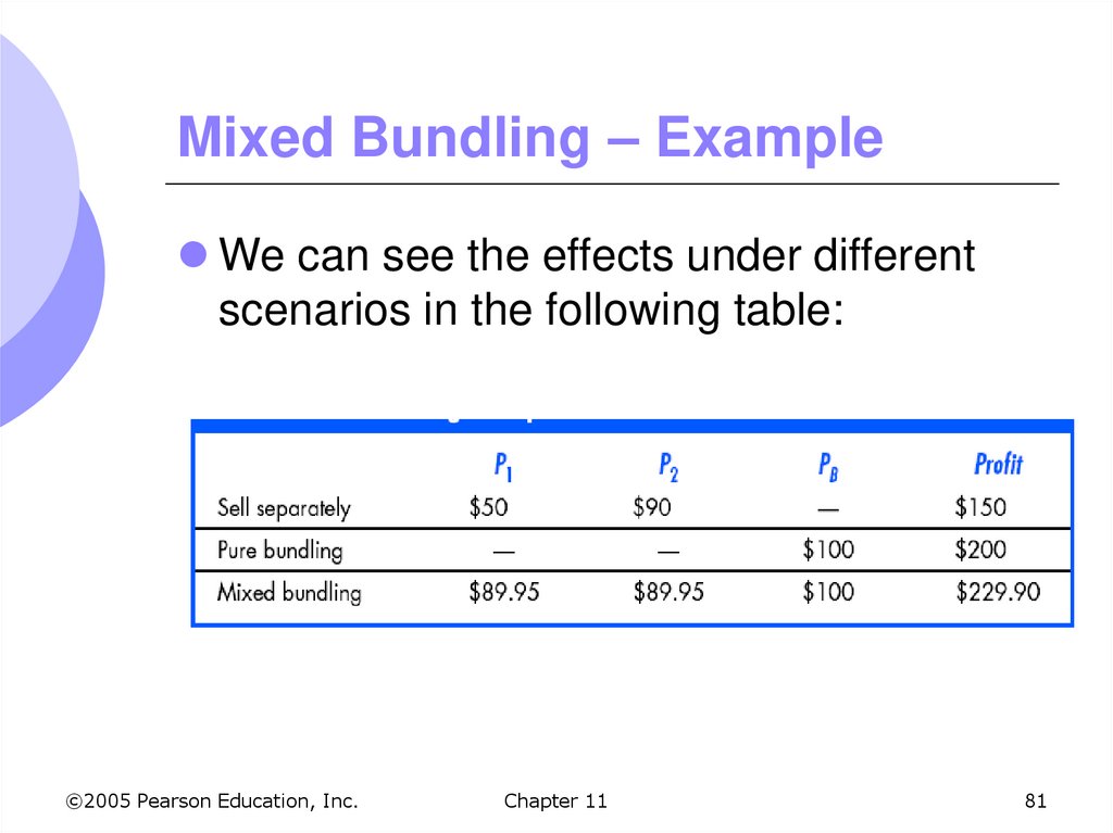
81. Mixed Bundling – Example

We can see the effects under different
scenarios in the following table:
©2005 Pearson Education, Inc.
Chapter 11
81

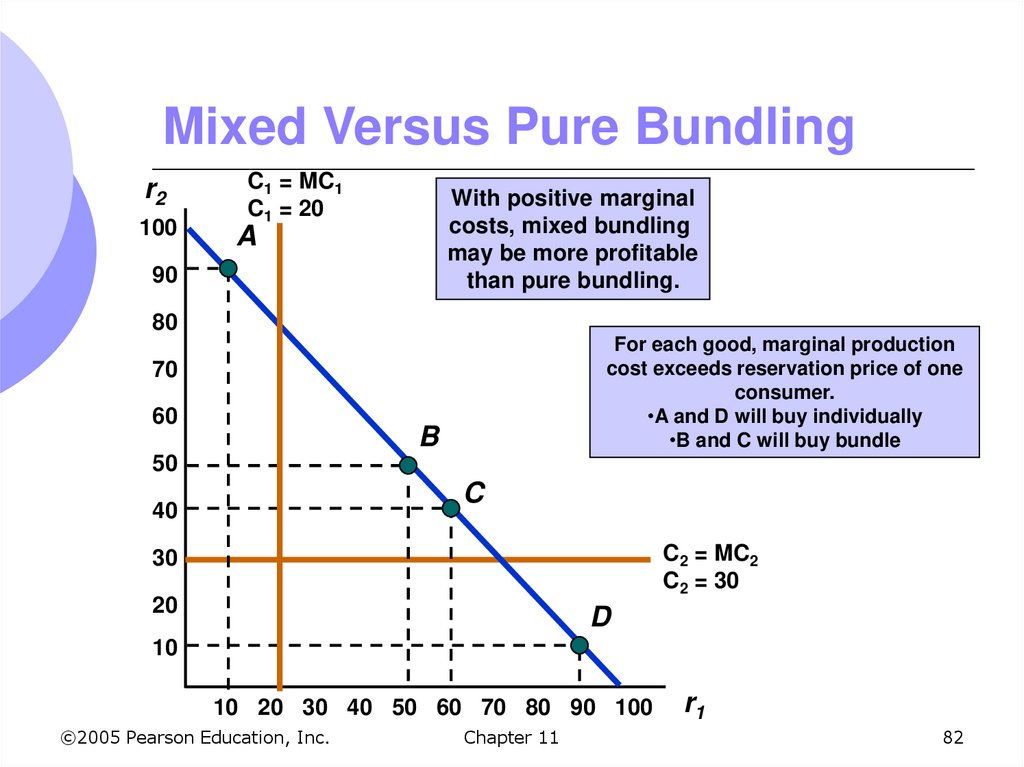
82. Mixed Versus Pure Bundling

r2
100
C1 = MC1
C1 = 20
With positive marginal
costs, mixed bundling
may be more profitable
than pure bundling.
A
90
80
For each good, marginal production
cost exceeds reservation price of one
consumer.
•A and D will buy individually
•B and C will buy bundle
70
60
B
50
C
40
C2 = MC2
C2 = 30
30
20
D
10
10 20 30 40 50 60 70 80 90 100
©2005 Pearson Education, Inc.
Chapter 11
r1
82

83. Bundling

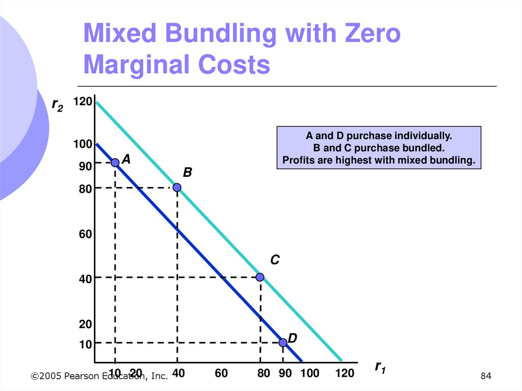
If MC is zero, mixed bundling can still be
more profitable if consumer demands are
not perfectly negatively correlated
Example:
Reservation prices for consumers B and C
are higher
Compare the same three strategies
Mixed bundling is the more profitable option
since everyone will end up buying
©2005 Pearson Education, Inc.
Chapter 11
83

84. Mixed Bundling with Zero Marginal Costs

r2
120
A and D purchase individually.
B and C purchase bundled.
Profits are highest with mixed bundling.
100
90
A
B
80
60
C
40
20
D
10
10 20 Inc. 40
©2005 Pearson Education,
60
80 90 100
120
r1
84

85. Bundling in Practice

Car purchasing
Bundles of options such as electric locks with
air conditioning
Vacation Travel
Bundling hotel with air fare
Cable television
Premium channels bundled together
©2005 Pearson Education, Inc.
Chapter 11
85

86. Bundling

Mixed Bundling in Practice
Use of market surveys to determine
reservation prices
Design a pricing strategy from the survey
results
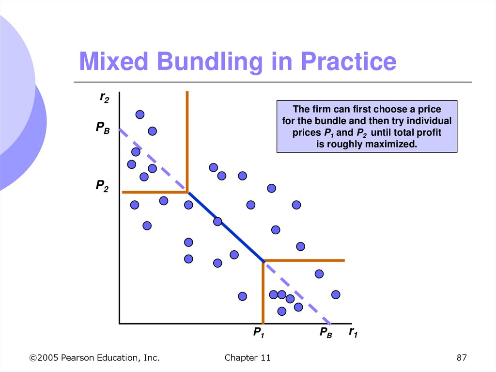
Can show graphically using information
collected from consumers
Consumers are separated into four regions
Can change prices to find max profits
©2005 Pearson Education, Inc.
Chapter 11
86

87. Mixed Bundling in Practice

r2
The firm can first choose a price
for the bundle and then try individual
prices P1 and P2 until total profit
is roughly maximized.
PB
P2
P1
©2005 Pearson Education, Inc.
Chapter 11
PB
r1
87

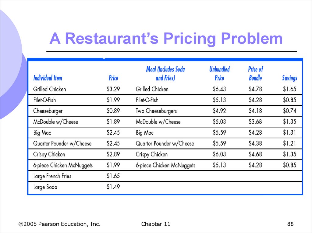
88. A Restaurant’s Pricing Problem

©2005 Pearson Education, Inc.
Chapter 11
88

89. Tying

The practice of requiring a customer to
purchase one good in order to purchase
another
Xerox machines and the paper
IBM mainframe and computer cards
Allows firm to meter demand and practice
price discrimination more effectively
©2005 Pearson Education, Inc.
Chapter 11
89

90. Tying

Allows the seller to meter the customer
and use a two-part tariff to discriminate
against the heavy user
McDonald’s
Allows them to protect their brand name
Microsoft
Uses to extend market power
©2005 Pearson Education, Inc.
Chapter 11
90

91. Advertising

Firms with market power have to decide
how much to advertise
We can show how firms choose profit
maximizing advertising
Decision depends on characteristics of
demand for firm’s product
©2005 Pearson Education, Inc.
Chapter 11
91

92. Advertising

Assumptions
Firm sets only one price for product
Firm knows quantity demanded depends on
price and advertising expenditure dollars, A
Q(P,A)
We can show the firm’s cost curves, revenue
curves, and profits under advertising and no
advertising
©2005 Pearson Education, Inc.
Chapter 11
92

93. Effects of Advertising

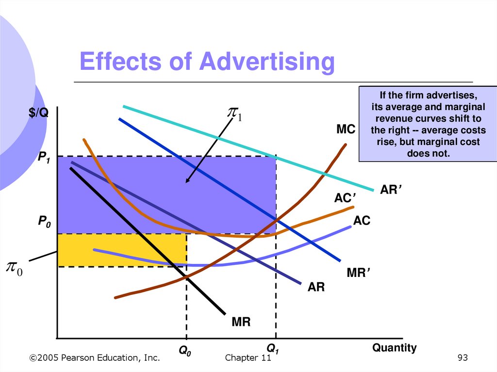
1
$/Q
MC
P1
AR
andfirm
MRadvertises,
are average
If the
and
revenue
when
its marginal
average and
marginal
the
firm doesn’t
revenue
curvesadvertise.
shift to
the right -- average costs
rise, but marginal cost
does not.
AC’
P0
AR’
AC
0
MR’
AR
MR
©2005 Pearson Education, Inc.
Q0
Q1
Chapter 11
Quantity
93

94. Advertising

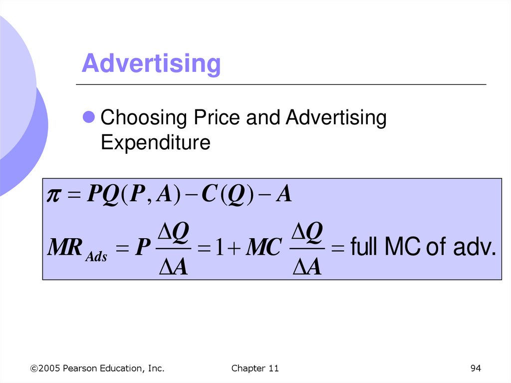
Choosing Price and Advertising
Expenditure
PQ( P , A) C (Q ) A
Q
Q
MR Ads P
1 MC
full MC of adv.
A
A
©2005 Pearson Education, Inc.
Chapter 11
94

95. Advertising

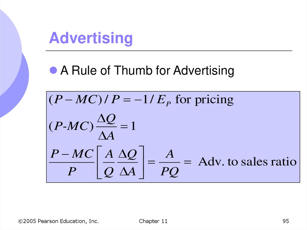
A Rule of Thumb for Advertising
( P MC ) / P 1 / E P for pricing
Q
( P-MC )
1
A
P MC A Q
A
Adv. to sales ratio
P
Q A PQ
©2005 Pearson Education, Inc.
Chapter 11
95

96. Advertising

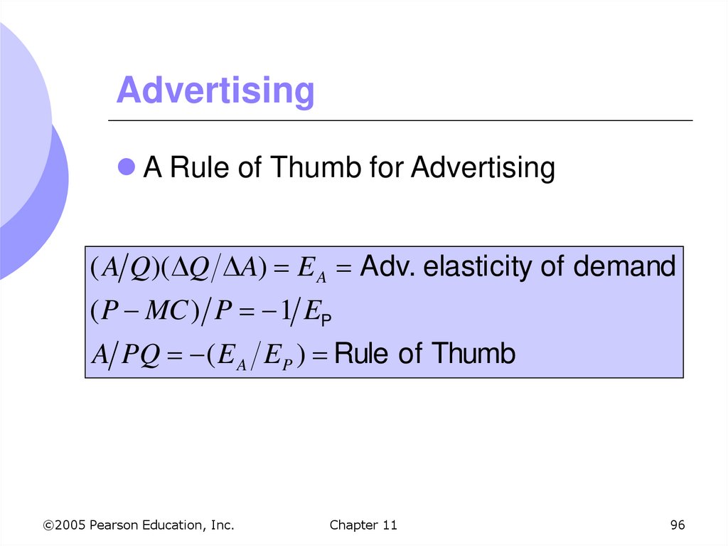
A Rule of Thumb for Advertising
( A Q)( Q A) E A Adv. elasticity of demand
( P MC ) P 1 EP
A PQ ( E A EP ) Rule of Thumb
©2005 Pearson Education, Inc.
Chapter 11
96

97. Advertising

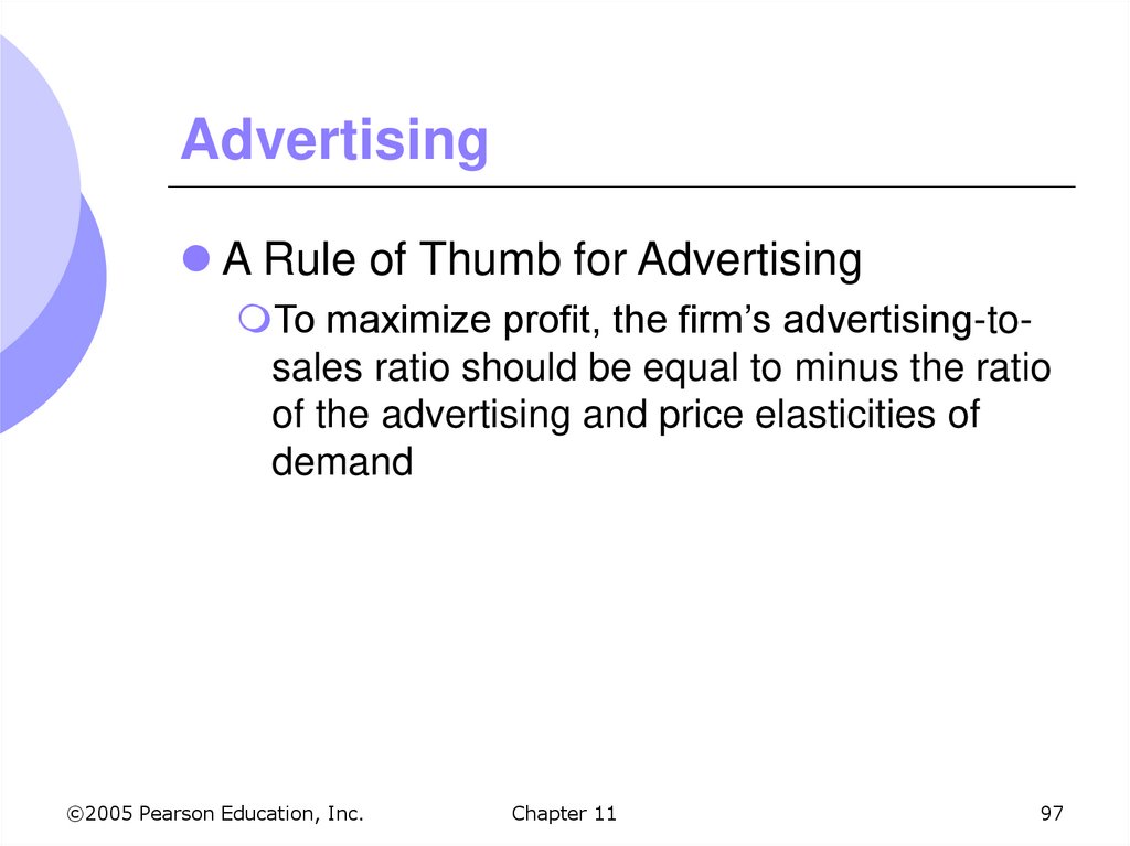
A Rule of Thumb for Advertising
To maximize profit, the firm’s advertising-tosales ratio should be equal to minus the ratio
of the advertising and price elasticities of
demand
©2005 Pearson Education, Inc.
Chapter 11
97

98. Advertising

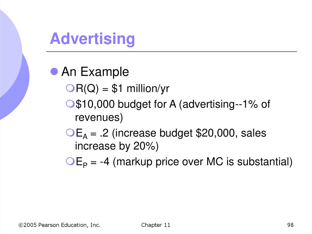
An Example
R(Q) = $1 million/yr
$10,000 budget for A (advertising--1% of
revenues)
EA = .2 (increase budget $20,000, sales
increase by 20%)
EP = -4 (markup price over MC is substantial)
©2005 Pearson Education, Inc.
Chapter 11
98

99. Advertising

The firm in our example should increase
advertising
A/PQ = -(2/-.4) = 5%
Increase budget to $50,000
©2005 Pearson Education, Inc.
Chapter 11
99

100. Advertising – In Practice

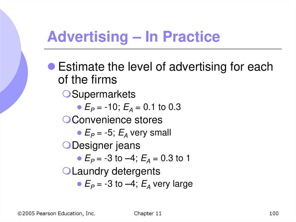
Estimate the level of advertising for each
of the firms
Supermarkets
EP = -10; EA = 0.1 to 0.3
Convenience stores
EP = -5; EA very small
Designer jeans
EP = -3 to –4; EA = 0.3 to 1
Laundry detergents
EP = -3 to –4; EA very large
©2005 Pearson Education, Inc.
Chapter 11
100