data analtics presentation

1. Data Analytics Project 1

Analysis of Large_Cars
By Sabrina Azimova
(80210)

2.

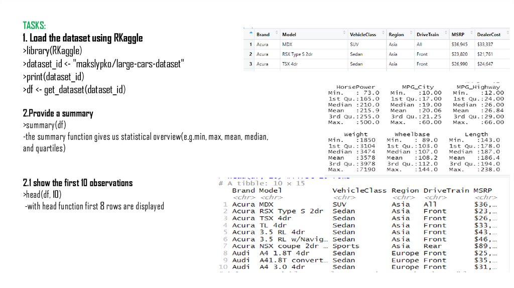
TASKS:
1. Load the dataset using RKaggle
>library(RKaggle)
>dataset_id <- "makslypko/large-cars-dataset"
>print(dataset_id)
>df <- get_dataset(dataset_id)
2.Provide a summary
>summary(df)
-the summary function gives us statistical overview(e.g.min, max, mean, median,
and quartiles)
2.1 show the first 10 observations
>head(df, 10)
-with head function first 8 rows are displayed

3.

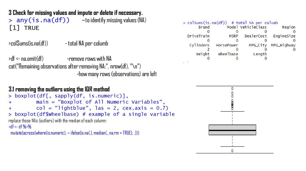
3 Check for missing values and impute or delete if necessary.
> any(is.na(df))
-to identify missing values (NA)
[1] TRUE
>colSums(is.na(df))
- total NA per columb
>df <- na.omit(df)
-remove rows with NA
cat("Remaining observations after removing NA:", nrow(df), "\n")
-how many rows (observations) are left
3.1 removing the outliers using the IQR method
> boxplot(df[, sapply(df, is.numeric)],
+
main = "Boxplot of All Numeric Variables",
+
col = "lightblue", las = 2, cex.axis = 0.7)
> boxplot(df$Wheelbase) # example of a single variable
replace those NAs (outliers) with the median of each column:
>df <- df %>%
mutate(across(where(is.numeric), ~ ifelse(is.na(.), median(., na.rm = TRUE), .)))

4.

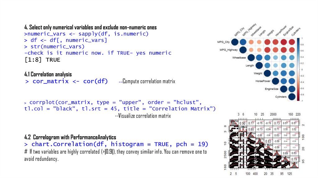
4. Select only numerical variables and exclude non-numeric ones
>numeric_vars <- sapply(df, is.numeric)
> df <- df[, numeric_vars]
> str(numeric_vars)
-check is it numeric now. if TRUE- yes numeric
[1:8] TRUE
4.1 Correlation analysis
> cor_matrix <- cor(df)
Compute correlation matrix
--
corrplot(cor_matrix, type = "upper", order = "hclust",
tl.col = "black", tl.srt = 45, title = "Correlation Matrix")
>
--Visualize correlation matrix
4.2 Correlogram with PerformanceAnalytics
> chart.Correlation(df, histogram = TRUE, pch = 19)
# If two variables are highly correlated (>|0.9|), they convey similar info. You can remove one to
avoid redundancy.

5.

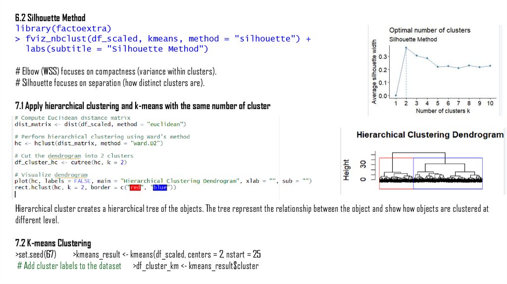
6.2 Silhouette Method
library(factoextra)
> fviz_nbclust(df_scaled, kmeans, method = "silhouette") +
labs(subtitle = "Silhouette Method")
# Elbow (WSS) focuses on compactness (variance within clusters).
# Silhouette focuses on separation (how distinct clusters are).
7.1 Apply hierarchical clustering and k-means with the same number of cluster
Hierarchical cluster creates a hierarchical tree of the objects. The tree represent the relationship between the object and show how objects are clustered at
different level.
7.2 K-means Clustering
>set.seed(67)
>kmeans_result <- kmeans(df_scaled, centers = 2, nstart = 25
# Add cluster labels to the dataset >df_cluster_km <- kmeans_result$cluster

6.

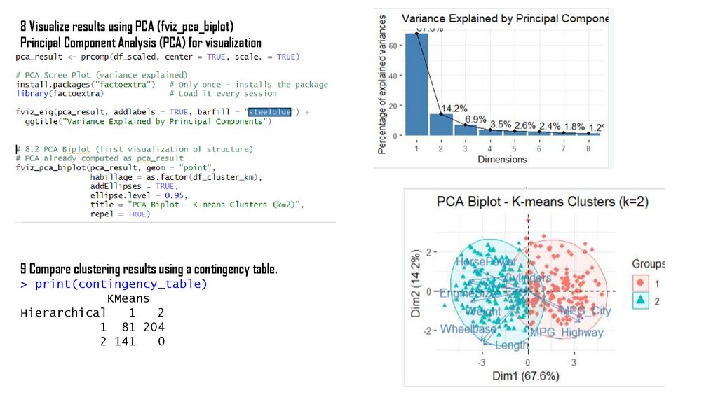
8 Visualize results using PCA (fviz_pca_biplot)
Principal Component Analysis (PCA) for visualization
9 Compare clustering results using a contingency table.
> print(contingency_table)
KMeans
Hierarchical
1
2
1 81 204
2 141
0

7.

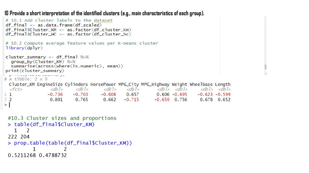
10 Provide a short interpretation of the identified clusters (e.g., main characteristics of each group).
#10.3 Cluster sizes and proportions
> table(df_final$Cluster_KM)
1
2
222 204
> prop.table(table(df_final$Cluster_KM))
1
2
0.5211268 0.4788732