Похожие презентации:
Statistics toolbox
1. Statistics toolbox
2. Decision Tree functions
treefittreeprune
treedisp
treetest
treeval
Fit a tree-based model for classification
or regression
Produce a sequence of subtrees by
pruning
Show classification or regression tree
graphically
Compute error rate for tree
Compute fitted value for decision tree
applied to data
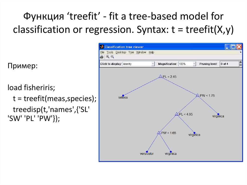
3. Функция ‘treefit’ - fit a tree-based model for classification or regression. Syntax: t = treefit(X,y)
Пример:load fisheriris;
t = treefit(meas,species);
treedisp(t,'names',{'SL'
'SW' 'PL' 'PW'});
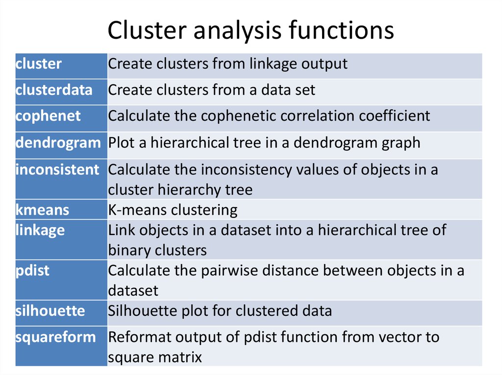
4. Cluster analysis functions
clusterCreate clusters from linkage output
clusterdata Create clusters from a data set
cophenet
Calculate the cophenetic correlation coefficient
dendrogram Plot a hierarchical tree in a dendrogram graph
inconsistent Calculate the inconsistency values of objects in a
cluster hierarchy tree
kmeans
K-means clustering
linkage
Link objects in a dataset into a hierarchical tree of
binary clusters
pdist
Calculate the pairwise distance between objects in a
dataset
silhouette Silhouette plot for clustered data
squareform Reformat output of pdist function from vector to
square matrix
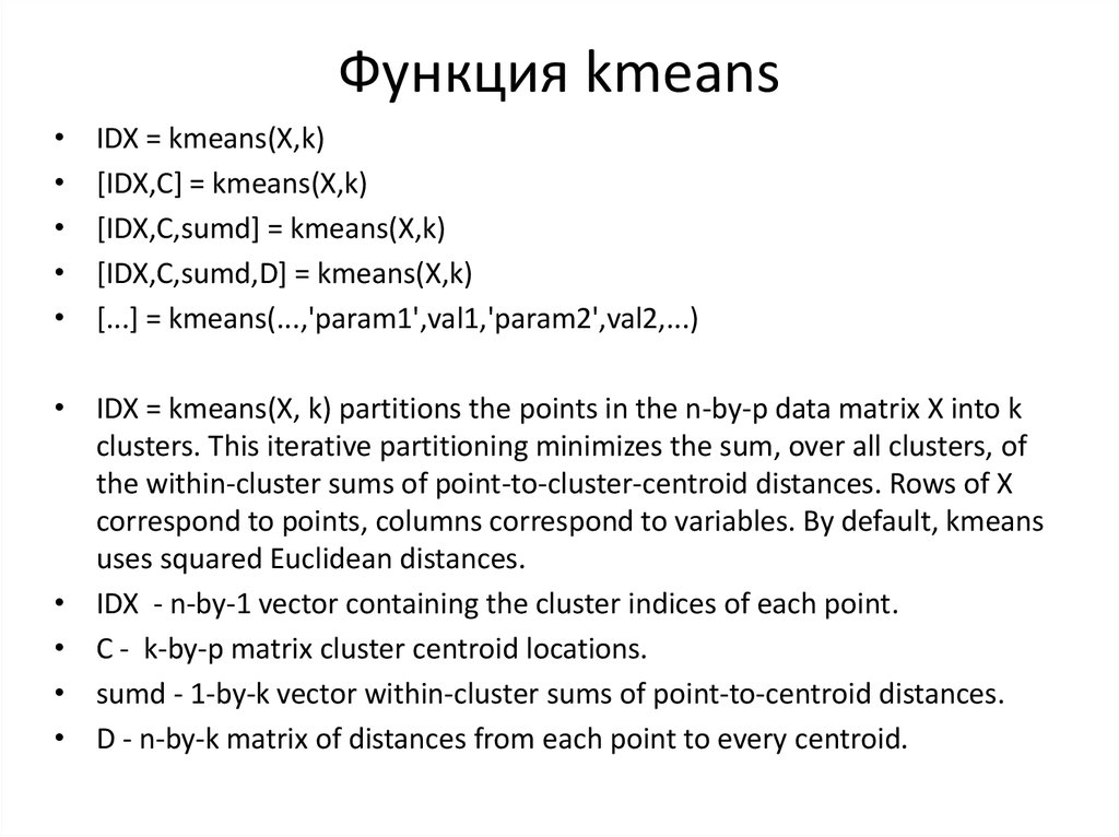
5. Функция kmeans
IDX = kmeans(X,k)
[IDX,C] = kmeans(X,k)
[IDX,C,sumd] = kmeans(X,k)
[IDX,C,sumd,D] = kmeans(X,k)
[...] = kmeans(...,'param1',val1,'param2',val2,...)
• IDX = kmeans(X, k) partitions the points in the n-by-p data matrix X into k
clusters. This iterative partitioning minimizes the sum, over all clusters, of
the within-cluster sums of point-to-cluster-centroid distances. Rows of X
correspond to points, columns correspond to variables. By default, kmeans
uses squared Euclidean distances.
• IDX - n-by-1 vector containing the cluster indices of each point.
• C - k-by-p matrix cluster centroid locations.
• sumd - 1-by-k vector within-cluster sums of point-to-centroid distances.
• D - n-by-k matrix of distances from each point to every centroid.
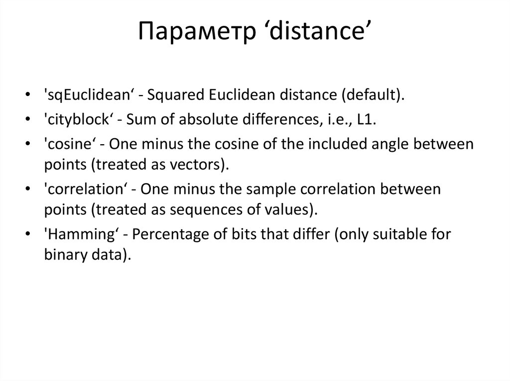
6. Параметр ‘distance’
• 'sqEuclidean‘ - Squared Euclidean distance (default).• 'cityblock‘ - Sum of absolute differences, i.e., L1.
• 'cosine‘ - One minus the cosine of the included angle between
points (treated as vectors).
• 'correlation‘ - One minus the sample correlation between
points (treated as sequences of values).
• 'Hamming‘ - Percentage of bits that differ (only suitable for
binary data).
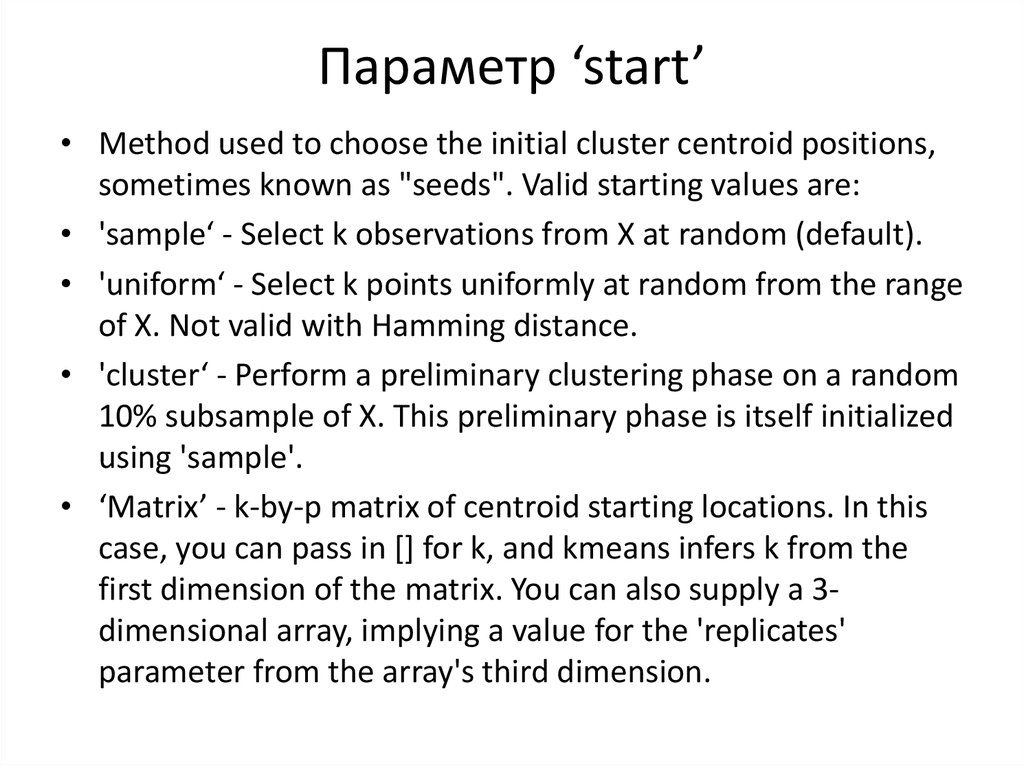
7. Параметр ‘start’
• Method used to choose the initial cluster centroid positions,sometimes known as "seeds". Valid starting values are:
• 'sample‘ - Select k observations from X at random (default).
• 'uniform‘ - Select k points uniformly at random from the range
of X. Not valid with Hamming distance.
• 'cluster‘ - Perform a preliminary clustering phase on a random
10% subsample of X. This preliminary phase is itself initialized
using 'sample'.
• ‘Matrix’ - k-by-p matrix of centroid starting locations. In this
case, you can pass in [] for k, and kmeans infers k from the
first dimension of the matrix. You can also supply a 3dimensional array, implying a value for the 'replicates'
parameter from the array's third dimension.
8. Classification
4.54
Sepal width
load fisheriris;
gscatter(meas(:,1),
meas(:,2),
species,'rgb','osd');
xlabel('Sepal length');
ylabel('Sepal width');
setosa
versicolor
virginica
3.5
3
2.5
2
4
4.5
5
5.5
6
6.5
Sepal length
7
7.5
8
9. Linear and quadratic discriminant analysis
Sepal widthlinclass = classify(meas(:,1:2),
meas(:,1:2),species);
4.5
bad = ~strcmp(linclass,species);
numobs = size(meas,1);
4
pbad = sum(bad) / numobs;
setosa
versicolor
virginica
3.5
hold on;
3
plot(meas(bad,1), meas(bad,2),
2.5
'kx');
hold off;
2
4
4.5
5
5.5
6
6.5
Sepal length
7
7.5
8
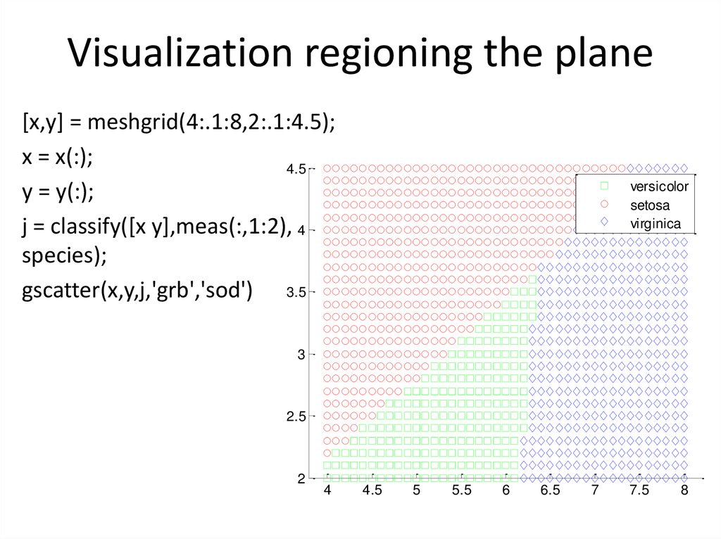
10. Visualization regioning the plane
[x,y] = meshgrid(4:.1:8,2:.1:4.5);x = x(:);
4.5
y = y(:);
j = classify([x y],meas(:,1:2), 4
species);
gscatter(x,y,j,'grb','sod') 3.5
y
versicolor
setosa
virginica
3
2.5
2
4
4.5
5
5.5
6
x
6.5
7
7.5
8
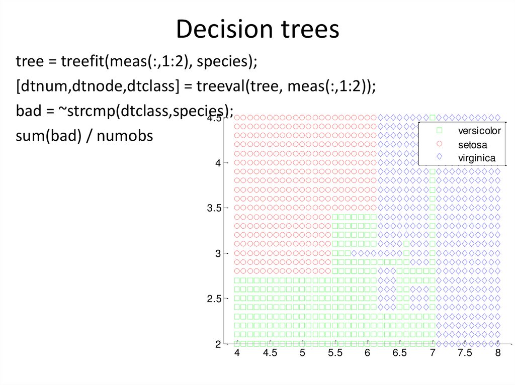
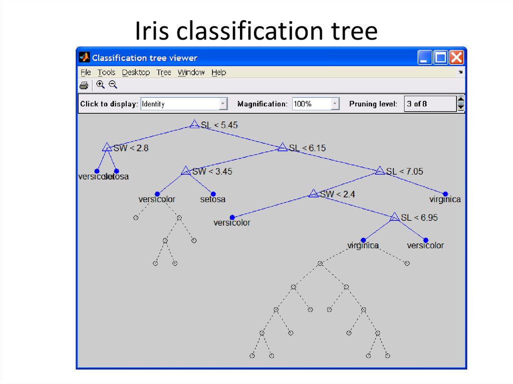
11. Decision trees
tree = treefit(meas(:,1:2), species);[dtnum,dtnode,dtclass] = treeval(tree, meas(:,1:2));
bad = ~strcmp(dtclass,species);
4.5
sum(bad) / numobs
versicolor
setosa
virginica
4
y
3.5
3
2.5
2
4
4.5
5
5.5
6
x
6.5
7
7.5
8
12. Iris classification tree
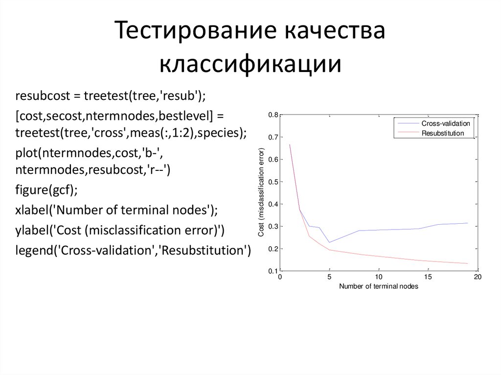
13. Тестирование качества классификации
0.8Cross-validation
Resubstitution
0.7
Cost (misclassification error)
resubcost = treetest(tree,'resub');
[cost,secost,ntermnodes,bestlevel] =
treetest(tree,'cross',meas(:,1:2),species);
plot(ntermnodes,cost,'b-',
ntermnodes,resubcost,'r--')
figure(gcf);
xlabel('Number of terminal nodes');
ylabel('Cost (misclassification error)')
legend('Cross-validation','Resubstitution')
0.6
0.5
0.4
0.3
0.2
0.1
0
5
10
15
Number of terminal nodes
20
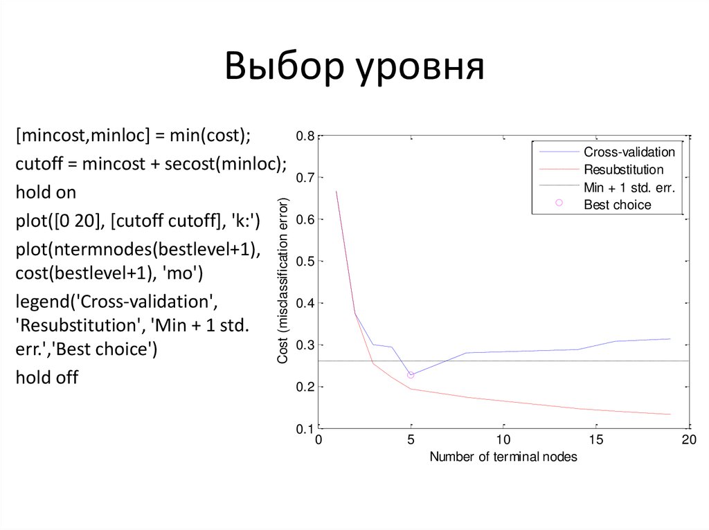
14. Выбор уровня
Cost (misclassification error)[mincost,minloc] = min(cost);
cutoff = mincost + secost(minloc);
hold on
plot([0 20], [cutoff cutoff], 'k:')
plot(ntermnodes(bestlevel+1),
cost(bestlevel+1), 'mo')
legend('Cross-validation',
'Resubstitution', 'Min + 1 std.
err.','Best choice')
hold off
0.8
Cross-validation
Resubstitution
Min + 1 std. err.
Best choice
0.7
0.6
0.5
0.4
0.3
0.2
0.1
0
5
10
15
Number of terminal nodes
20
15. Оптимальное дерево классификации
prunedtree = treeprune(tree,bestlevel);treedisp(prunedtree)
cost(bestlevel+1)
>> ans = 0.22
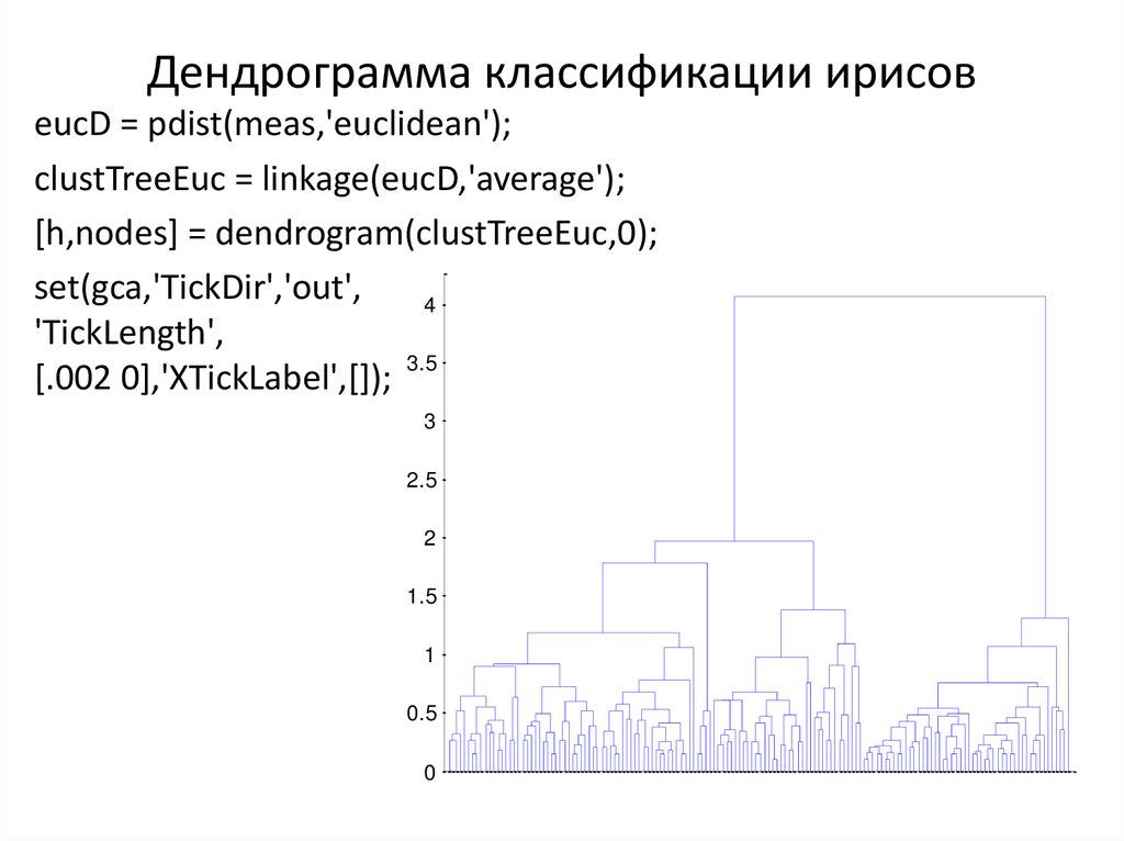
16. Дендрограмма классификации ирисов
eucD = pdist(meas,'euclidean');clustTreeEuc = linkage(eucD,'average');
[h,nodes] = dendrogram(clustTreeEuc,0);
set(gca,'TickDir','out',
4
'TickLength',
[.002 0],'XTickLabel',[]); 3.5
3
2.5
2
1.5
1
0.5
0




 Информатика


