Lecture 2_additional

1. Deep Neural Networks

Lecture 2: Gradient Descent. Stochastic Gradient Descent Algorithm.
Marat Nurtas
PhD in Mathematical and Computer Modeling
Department of Mathematical and Computer Modeling
International Information Technology University, Almaty, Kazakhstan

2. Table of Contents:

• Simple intuition behind Neural networks
• Multi Layer Perceptron and its basics
• Steps involved in Neural Network methodology
• Visualizing steps for Neural Network working methodology
• Implementing NN using Numpy (Python)
• Implementing NN using R
• [Optional] Mathematical Perspective of Back Propagation
Algorithm

3.

4.

Neural Networks
Overview
•Gradient Descent forms the basis of Neural networks
•Neural networks can be implemented in both R and Python
using certain libraries and packages

5. Introduction

You can learn and practice a concept in two ways:
• Option 1: You can learn the entire theory on a particular subject
and then look for ways to apply those concepts. So, you read up
how an entire algorithm works, the maths behind it, its
assumptions, limitations and then you apply it. Robust but time
taking approach.
• Option 2: Start with simple basics and develop an intuition on the
subject. Next, pick a problem and start solving it. Learn the
concepts while you are solving the problem. Keep tweaking and
improving your understanding. So, you read up how to apply an
algorithm – go out and apply it. Once you know how to apply it,
try it around with different parameters, values, limits and develop
an understanding of the algorithm.

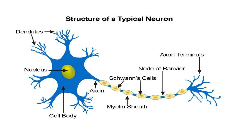
6. Simple intuition behind neural networks

.Neural networks work in very similar manner. It takes several input,
processes it through multiple neurons from multiple hidden layers and returns
the result using an output layer. This result estimation process is technically
known as “Forward Propagation“.
.Next, we compare the result with actual output. The task is to make the output
to neural network as close to actual (desired) output. Each of these neurons are
contributing some error to final output. How do you reduce the error?
.We try to minimize the value/ weight of neurons those are contributing more
to the error and this happens while traveling back to the neurons of the neural
network and finding where the error lies. This process is known as
“Backward Propagation“.
. In order to reduce these number of iterations to minimize the error, the neural
networks use a common algorithm known as “Gradient Descent”, which helps
to optimize the task quickly and efficiently.

7. Multi Layer Perceptron and its basics

Just like atoms form the basics of any material on earth – the basic forming
unit of a neural network is a perceptron. So, what is a perceptron?
• A perceptron can be understood as anything that takes multiple inputs and
produces one output.

8. three ways of creating input output relationships:

• By directly combining the input and computing the output based on a threshold
value. for eg: Take x1=0, x2=1, x3=1 and setting a threshold =0. So, if
x1+x2+x3>0, the output is 1 otherwise 0. You can see that in this case, the
perceptron calculates the output as 1.
• Next, let us add weights to the inputs. Weights give importance to an input. For
example, you assign w1=2, w2=3 and w3=4 to x1, x2 and x3 respectively. To
compute the output, we will multiply input with respective weights and compare
with threshold value as w1*x1 + w2*x2 + w3*x3 > threshold. These weights
assign more importance to x3 in comparison to x1 and x2.
• Next, let us add bias: Each perceptron also has a bias which can be thought of as
how much flexible the perceptron is. It is somehow similar to the constant b of a
linear function y = ax + b. It allows us to move the line up and down to fit the
prediction with the data better. Without b the line will always goes through the
origin (0, 0) and you may get a poorer fit. For example, a perceptron may have two
inputs, in that case, it requires three weights. One for each input and one for the
bias. Now linear representation of input will look like, w1*x1 + w2*x2 + w3*x3 +
1*b.

9. What is an activation function?

Activation Function takes the sum of weighted input
(w1*x1 + w2*x2 + w3*x3 + 1*b) as an argument and
return the output of the neuron.
In above equation, we have represented 1 as x0 and b as w0.
The activation function is mostly used to make a non-linear
transformation which allows us to fit nonlinear hypotheses or to
estimate the complex functions. There are multiple activation
functions, like: “Sigmoid”, “Tanh”, ReLu and many other.

10. Forward Propagation, Back Propagation and Epochs

• Till now, we have computed the output and this process is known as
“Forward Propagation“. But what if the estimated output is far
away from the actual output (high error). In the neural network
what we do, we update the biases and weights based on the error.
This weight and bias updating process is known as “Back
Propagation“.
• Back-propagation (BP) algorithms work by determining the loss (or
error) at the output and then propagating it back into the network.
The weights are updated to minimize the error resulting from each
neuron. The first step in minimizing the error is to determine the
gradient (Derivatives) of each node w.r.t. the final output.
• Note: This one round of forward and back propagation iteration is known as one training iteration aka
“Epoch“.

11. Multi-layer perceptron

• We have seen just a single layer consisting of 3 input nodes i.e x1, x2 and
x3 and an output layer consisting of a single neuron. But, for practical
purposes, the single-layer network can do only so much. An MLP consists
of multiple layers called Hidden Layers stacked in between the Input
Layer and the Output Layer.

12. Full Batch Gradient Descent and Stochastic Gradient Descent

• Both variants of Gradient Descent perform the same work of updating the
weights of the MLP by using the same updating algorithm but the difference
lies in the number of training samples used to update the weights and
biases.
• Full Batch Gradient Descent Algorithm as the name implies uses all the
training data points to update each of the weights once whereas Stochastic
Gradient uses 1 or more(sample) but never the entire training data to
update the weights once.
• Let us understand this with a simple example of a dataset of 10 data
points with two weights w1 and w2.
• Full Batch: You use 10 data points (entire training data) and calculate the
change in w1 (Δw1) and change in w2(Δw2) and update w1 and w2.
• SGD: You use 1st data point and calculate the change in w1 (Δw1) and
change in w2(Δw2) and update w1 and w2. Next, when you use 2nd data
point, you will work on the updated weights

13. Steps involved in Neural Network methodology

Steps involved in Neural Network methodology
• First look at the broad steps:
0.) We take input and output
• X as an input matrix
• y as an output matrix
1.) We initialize weights and biases with random values (This is one time initiation. In
the next iteration, we will use updated weights, and biases). Let us define:
• wh as weight matrix to the hidden layer
• bh as bias matrix to the hidden layer
• wout as weight matrix to the output layer
• bout as bias matrix to the output layer
Note: At the output layer, we have only one neuron as we are solving a binary classification problem (predict 0 or 1).
We could also have two neurons for predicting each of both classes.

14.

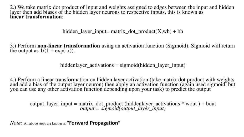
2.) We take matrix dot product of input and weights assigned to edges between the input and hidden
layer then add biases of the hidden layer neurons to respective inputs, this is known as
linear transformation:
hidden_layer_input= matrix_dot_product(X,wh) + bh
3.) Perform non-linear transformation using an activation function (Sigmoid). Sigmoid will return
the output as 1/(1 + exp(-x)).
hiddenlayer_activations = sigmoid(hidden_layer_input)
4.) Perform a linear transformation on hidden layer activation (take matrix dot product with weights
and add a bias of the output layer neuron) then apply an activation function (again used sigmoid, but
you can use any other activation function depending upon your task) to predict the output
output_layer_input = matrix_dot_product (hiddenlayer_activations * wout ) + bout
output = sigmoid(output_layer_input)
Note: All above steps are known as “Forward Propagation“

15.

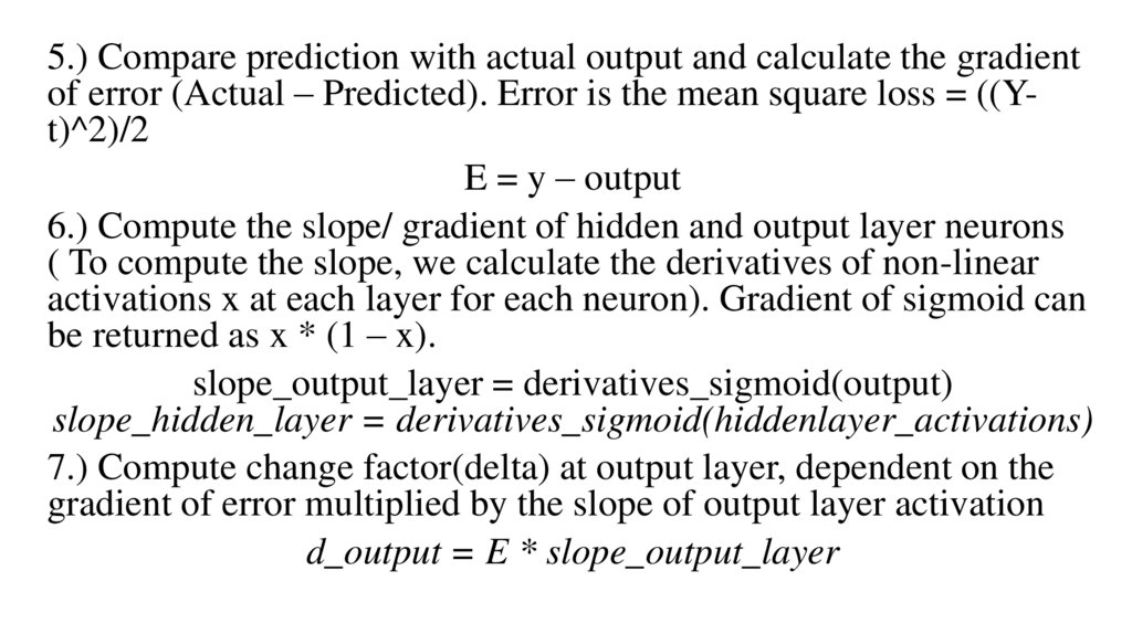
5.) Compare prediction with actual output and calculate the gradient
of error (Actual – Predicted). Error is the mean square loss = ((Yt)^2)/2
E = y – output
6.) Compute the slope/ gradient of hidden and output layer neurons
( To compute the slope, we calculate the derivatives of non-linear
activations x at each layer for each neuron). Gradient of sigmoid can
be returned as x * (1 – x).
slope_output_layer = derivatives_sigmoid(output)
slope_hidden_layer = derivatives_sigmoid(hiddenlayer_activations)
7.) Compute change factor(delta) at output layer, dependent on the
gradient of error multiplied by the slope of output layer activation
d_output = E * slope_output_layer

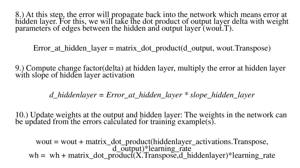
16.

8.) At this step, the error will propagate back into the network which means error at
hidden layer. For this, we will take the dot product of output layer delta with weight
parameters of edges between the hidden and output layer (wout.T).
Error_at_hidden_layer = matrix_dot_product(d_output, wout.Transpose)
9.) Compute change factor(delta) at hidden layer, multiply the error at hidden layer
with slope of hidden layer activation
d_hiddenlayer = Error_at_hidden_layer * slope_hidden_layer
10.) Update weights at the output and hidden layer: The weights in the network can
be updated from the errors calculated for training example(s).
wout = wout + matrix_dot_product(hiddenlayer_activations.Transpose,
d_output)*learning_rate
wh = wh + matrix_dot_product(X.Transpose,d_hiddenlayer)*learning_rate

17.

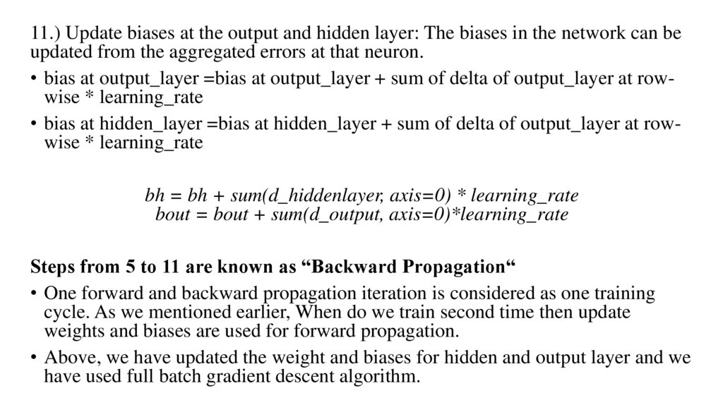
11.) Update biases at the output and hidden layer: The biases in the network can be
updated from the aggregated errors at that neuron.
• bias at output_layer =bias at output_layer + sum of delta of output_layer at rowwise * learning_rate
• bias at hidden_layer =bias at hidden_layer + sum of delta of output_layer at rowwise * learning_rate
bh = bh + sum(d_hiddenlayer, axis=0) * learning_rate
bout = bout + sum(d_output, axis=0)*learning_rate
Steps from 5 to 11 are known as “Backward Propagation“
• One forward and backward propagation iteration is considered as one training
cycle. As we mentioned earlier, When do we train second time then update
weights and biases are used for forward propagation.
• Above, we have updated the weight and biases for hidden and output layer and we
have used full batch gradient descent algorithm.

18. Visualization of steps for Neural Network methodology

Note:
• For good visualization images, We have rounded decimal positions at 2 or3 positions.
• Yellow filled cells represent current active cell
• Orange cell represents the input used to populate values of current cell
Step 0: Read input and output

19.

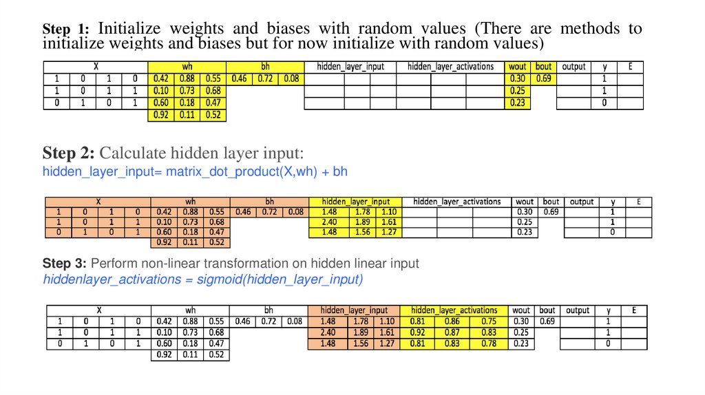
Step 1: Initialize weights and biases with random values (There are methods to
initialize weights and biases but for now initialize with random values)
Step 2: Calculate hidden layer input:
hidden_layer_input= matrix_dot_product(X,wh) + bh
Step 3: Perform non-linear transformation on hidden linear input
hiddenlayer_activations = sigmoid(hidden_layer_input)

20.

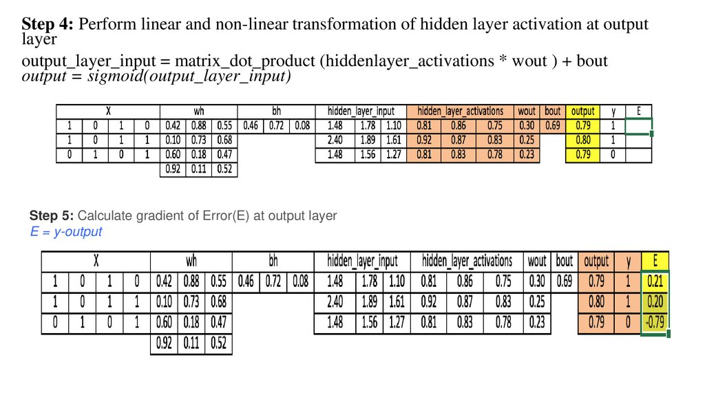
Step 4: Perform linear and non-linear transformation of hidden layer activation at output
layer
output_layer_input = matrix_dot_product (hiddenlayer_activations * wout ) + bout
output = sigmoid(output_layer_input)
Step 5: Calculate gradient of Error(E) at output layer
E = y-output

21.

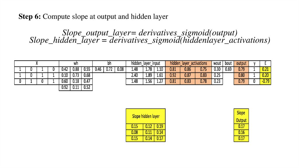
Step 6: Compute slope at output and hidden layer
Slope_output_layer= derivatives_sigmoid(output)
Slope_hidden_layer = derivatives_sigmoid(hiddenlayer_activations)

22.

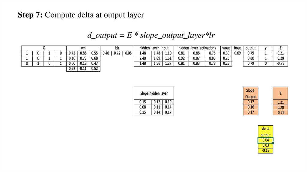
Step 7: Compute delta at output layer
d_output = E * slope_output_layer*lr

23.

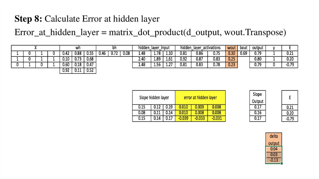
Step 8: Calculate Error at hidden layer
Error_at_hidden_layer = matrix_dot_product(d_output, wout.Transpose)

24.

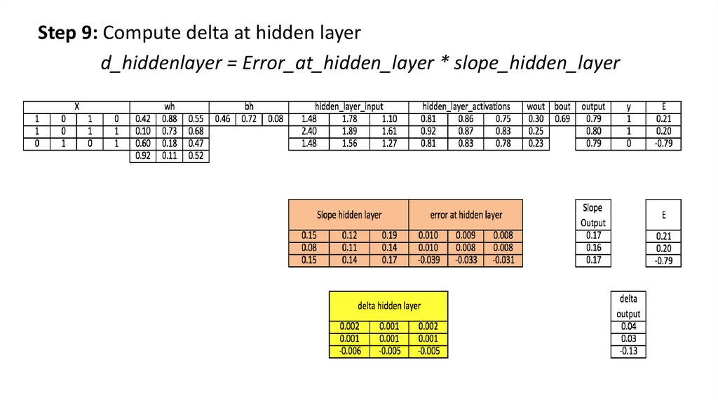
Step 9: Compute delta at hidden layer
d_hiddenlayer = Error_at_hidden_layer * slope_hidden_layer

25.

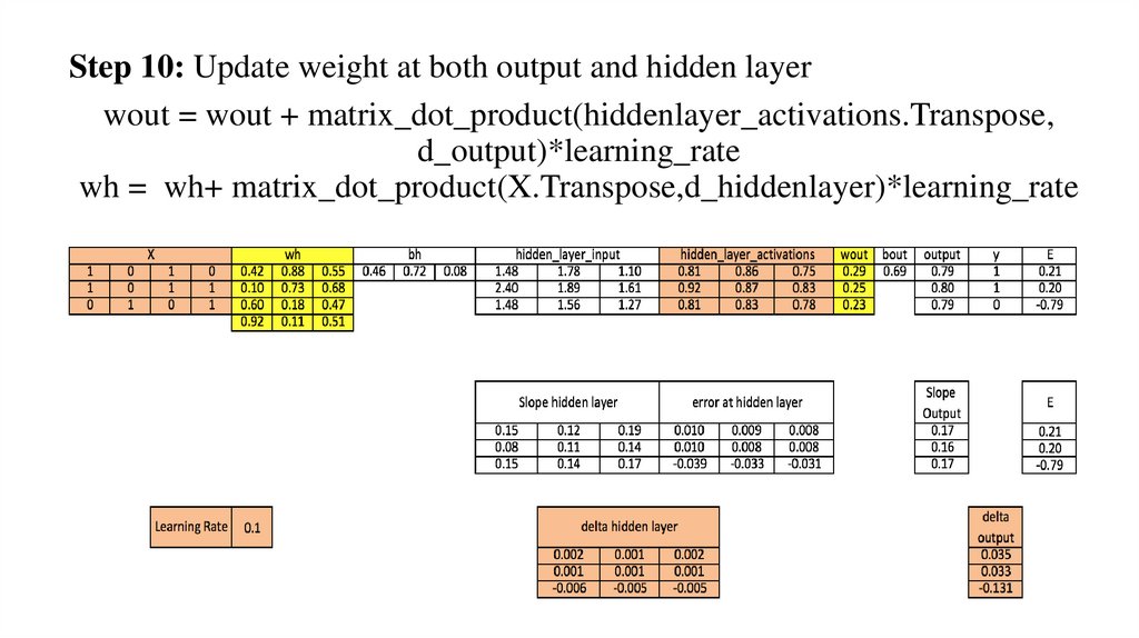
Step 10: Update weight at both output and hidden layer
wout = wout + matrix_dot_product(hiddenlayer_activations.Transpose,
d_output)*learning_rate
wh = wh+ matrix_dot_product(X.Transpose,d_hiddenlayer)*learning_rate

26.

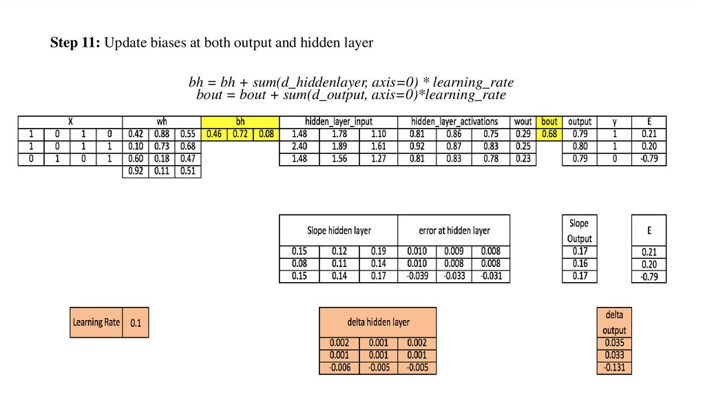
Step 11: Update biases at both output and hidden layer
bh = bh + sum(d_hiddenlayer, axis=0) * learning_rate
bout = bout + sum(d_output, axis=0)*learning_rate

27.

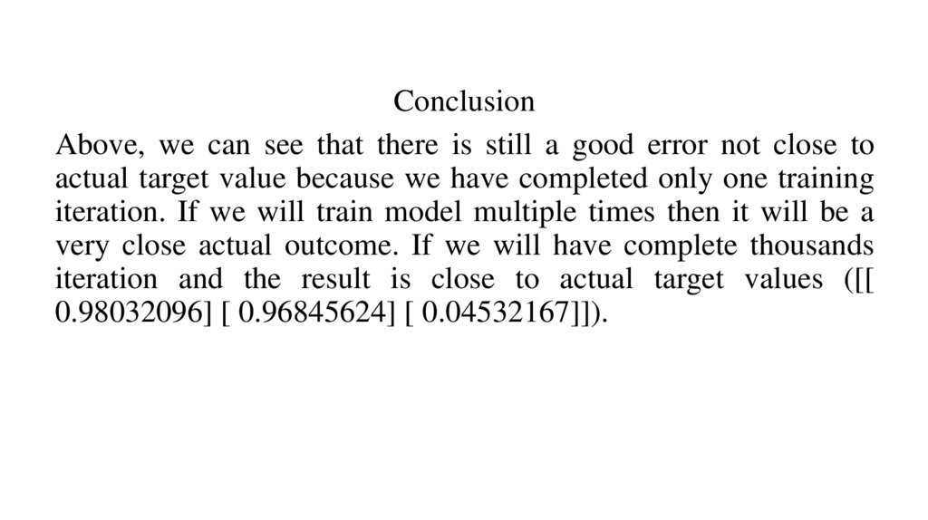
Conclusion
Above, we can see that there is still a good error not close to
actual target value because we have completed only one training
iteration. If we will train model multiple times then it will be a
very close actual outcome. If we will have complete thousands
iteration and the result is close to actual target values ([[
0.98032096] [ 0.96845624] [ 0.04532167]]).