Back propagation example

1.

19
back-propagation training

2.

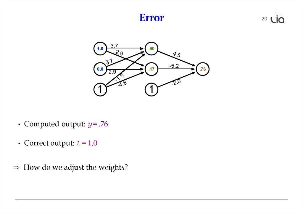
Error
1.0
0.0
3.7
2.9
1
• Computed output: y = .76
• Correct output: t = 1.0
⇒ How do we adjust the weights?
20
.90
.17
1
-5.2
.76

3.

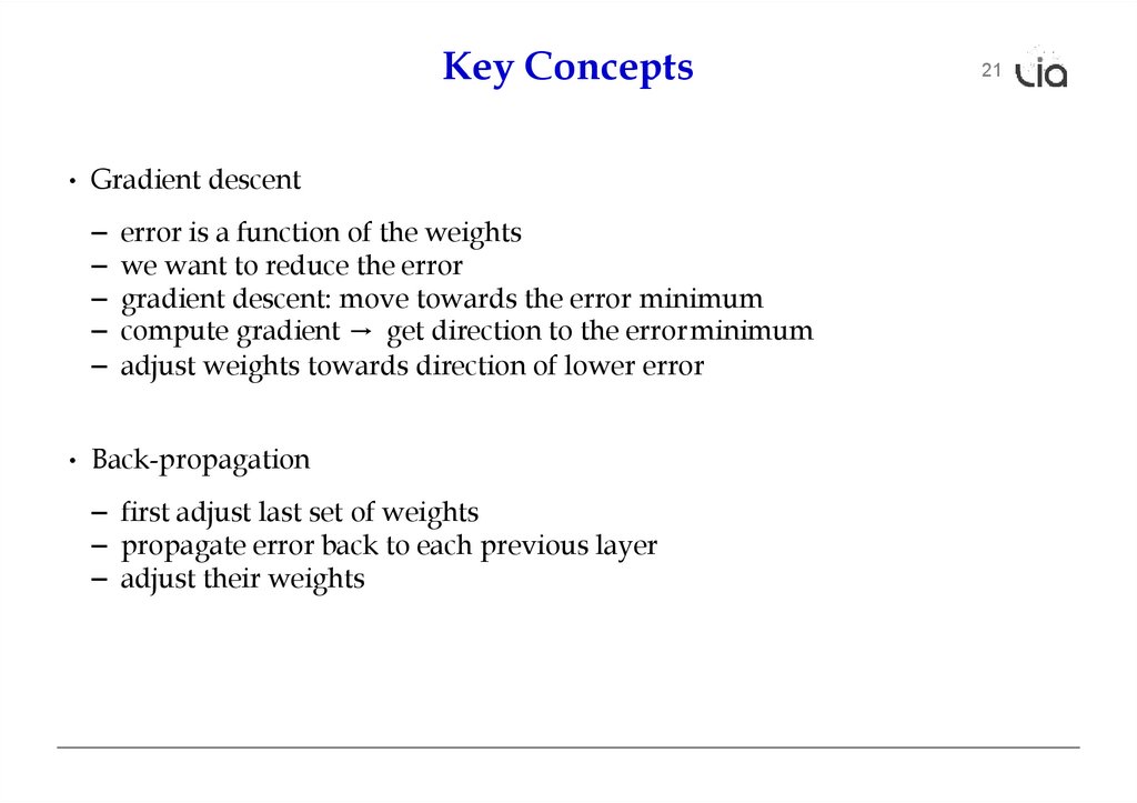
Key Concepts
• Gradient descent
–
–
–
–
–
error is a function of the weights
we want to reduce the error
gradient descent: move towards the error minimum
compute gradient → get direction to the error minimum
adjust weights towards direction of lower error
• Back-propagation
– first adjust last set of weights
– propagate error back to each previous layer
– adjust their weights
21

4.

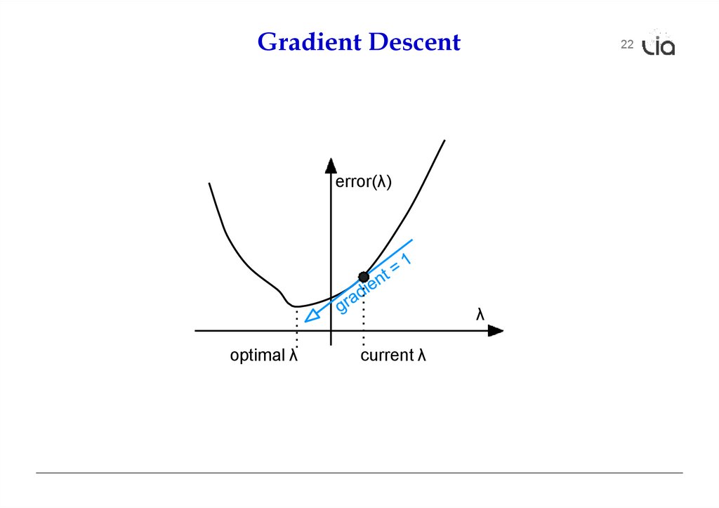
Gradient Descent
22
error(λ)
λ
optimal λ
current λ

5.

Gradient Descent
Gradient for w1
Current Point
Gradient for w2
Optimum
23

6.

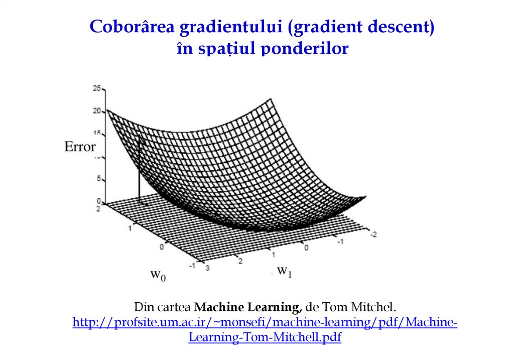
Coborârea gradientului (gradient descent)
în spațiul ponderilor
Din cartea Machine Learning, de Tom Mitchel.
http://profsite.um.ac.ir/~monsefi/machine-learning/pdf/MachineLearning-Tom-Mitchell.pdf

7.

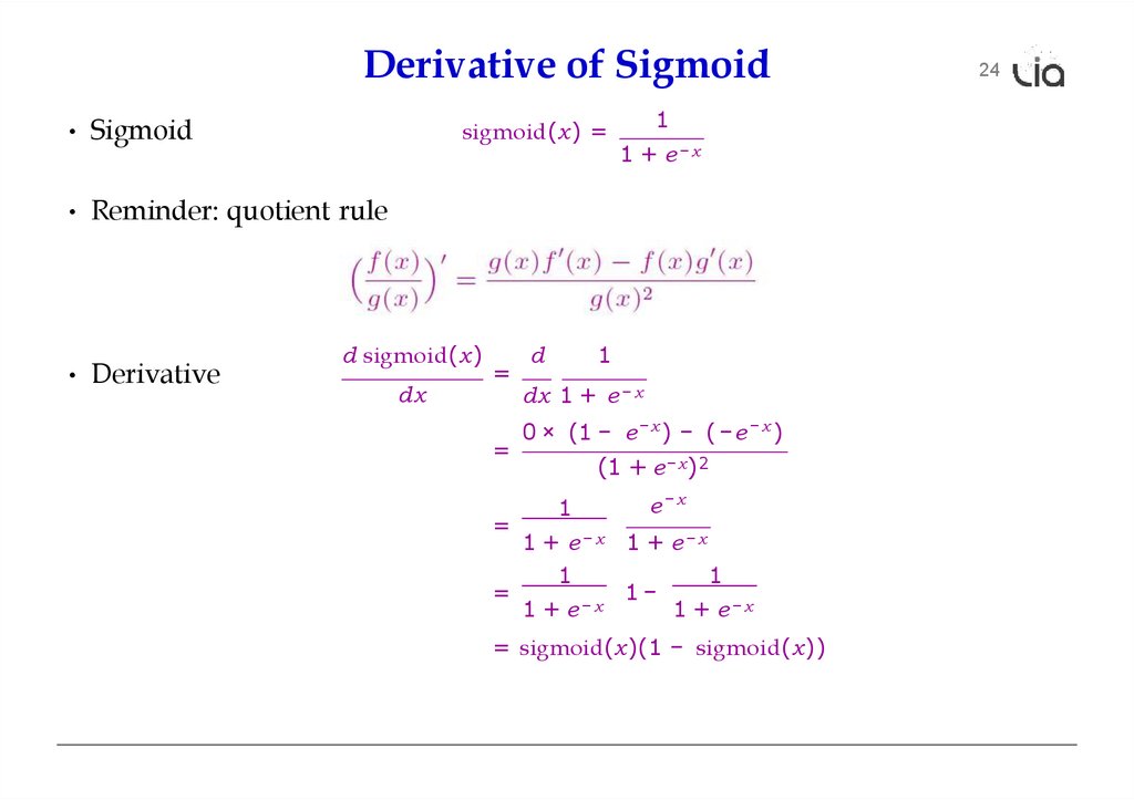
Derivative of Sigmoid
• Sigmoid
sigmoid(x) =
1
1 + e−x
• Reminder: quotient rule
• Derivative
d sigmoid(x)
dx
=
=
d
1
dx 1 + e − x
0 × (1 − e − x ) − ( − e − x )
(1 + e −x ) 2
e−x
1
=
1 + e−x 1 + e−x
1
1
1
−
=
1 + e−x
1 + e−x
= sigmoid(x)(1 − sigmoid(x))
24

8.

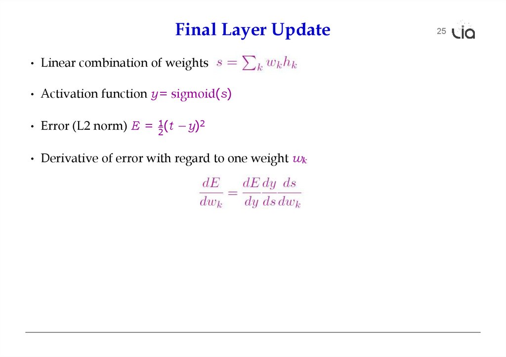
Final Layer Update
• Linear combination of weights
• Activation function y = sigmoid(s)
• Error (L2 norm) E = 12(t −y)2
• Derivative of error with regard to one weight wk
25

9.

Final Layer Update (1)
• Linear combination of weights
• Activation function y = sigmoid(s)
• Error (L2 norm) E = 12(t −y)2
• Derivative of error with regard to one weight wk
dE
dE dy ds
=
dwk
dy dsdwk
• Error E is defined with respect to y
2
26

10.

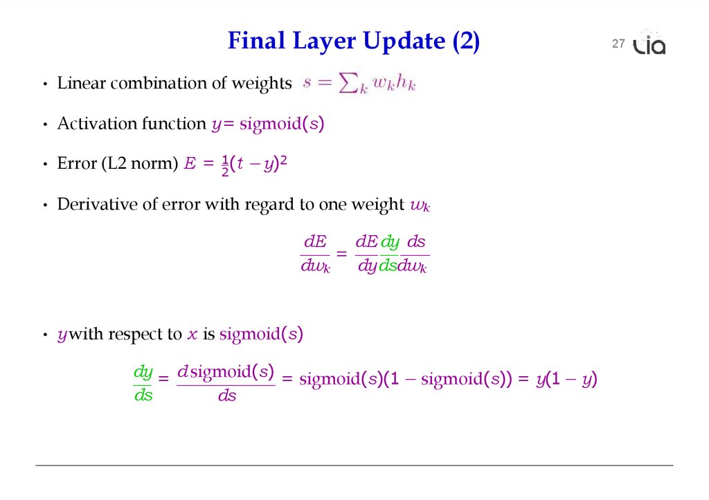
Final Layer Update (2)
• Linear combination of weights
• Activation function y = sigmoid(s)
• Error (L2 norm) E = 12(t −y)2
• Derivative of error with regard to one weight wk
dE
dE dy ds
=
dwk
dy dsdwk
• y with respect to x is sigmoid(s)
dy = d sigmoid(s) = sigmoid(s)(1 − sigmoid(s)) = y(1 − y)
ds
ds
27

11.

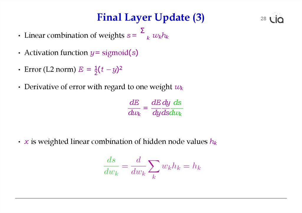
Final Layer Update (3)
• Linear combination of weights s =
Σ
k
wkhk
• Activation function y = sigmoid(s)
• Error (L2 norm) E = 12(t −y)2
• Derivative of error with regard to one weight wk
dE
dE dy ds
=
dwk
dy dsdwk
• x is weighted linear combination of hidden node values hk
28

12.

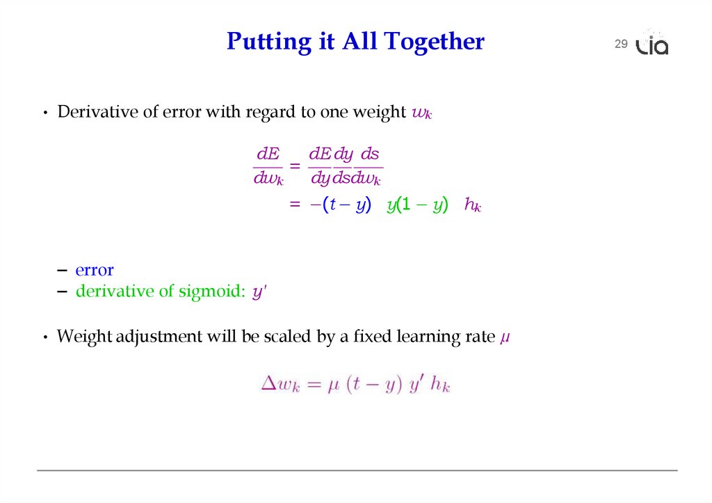
Putting it All Together
• Derivative of error with regard to one weight wk
dE
dE dy ds
=
dwk
dy dsdwk
= −(t − y) y(1 − y) hk
– error
– derivative of sigmoid: y'
• Weight adjustment will be scaled by a fixed learning rate µ
29

13.

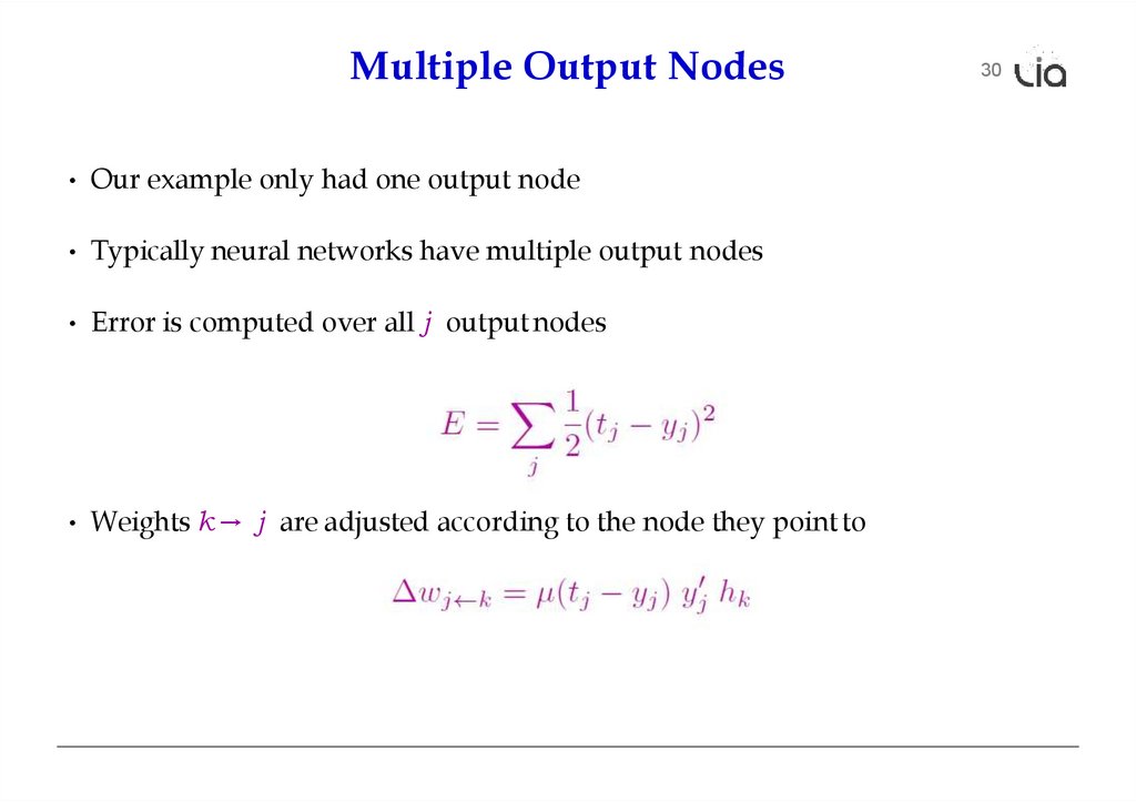
Multiple Output Nodes
• Our example only had one output node
• Typically neural networks have multiple output nodes
• Error is computed over all j output nodes
• Weights k → j are adjusted according to the node they point to
30

14.

Hidden Layer Update
31
• In a hidden layer, we do not have a target output value
• But we can compute how much each node contributed to downstream error
• Definition of error term of each node
• Back-propagate the error term
(why this way? there is math to back it up...)
• Universal update formula
∆w j←k = µ δj hk

15.

Our Example
A
1.0
3.7
D
.90
G
E
B
0.0
C
.17
2.9
-5.2
F
1
32
1
• Computed output: y = .76
• Correct output: t = 1.0
• Final layer weight updates (learning rate µ = 10)
– δG = (t − y) y' = (1 − .76) 0.181 = .0434
– ∆wGD = µ δG hD = 10 × .0434 × .90 = .391
– ∆wGE = µ δG hE = 10 × .0434 × .17 = .074
– ∆wGF = µ δG hF = 10 × .0434 × 1 = .434
.76

16.

Our Example
A
1.0
3.7
D
.90
E
B
0.0
C
.17
2.9
-5.126 -—5.—2
F
1
33
1
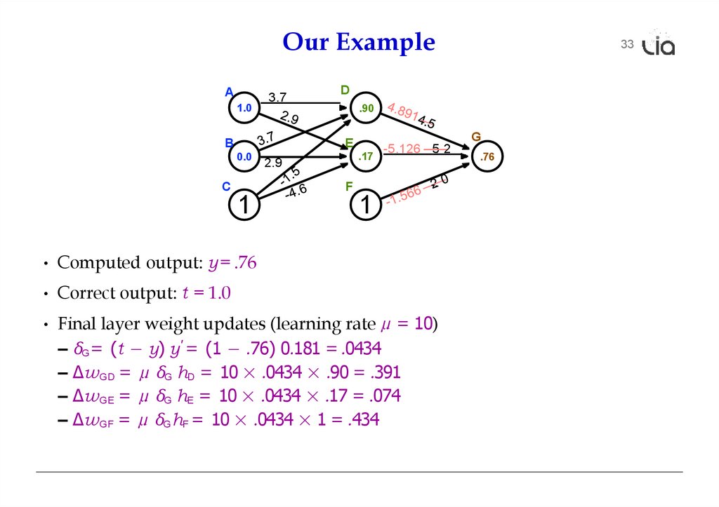
• Computed output: y = .76
• Correct output: t = 1.0
• Final layer weight updates (learning rate µ = 10)
– δG = (t − y) y' = (1 − .76) 0.181 = .0434
– ∆wGD = µ δG hD = 10 × .0434 × .90 = .391
– ∆wGE = µ δG hE = 10 × .0434 × .17 = .074
– ∆wGF = µ δG hF = 10 × .0434 × 1 = .434
G
.76

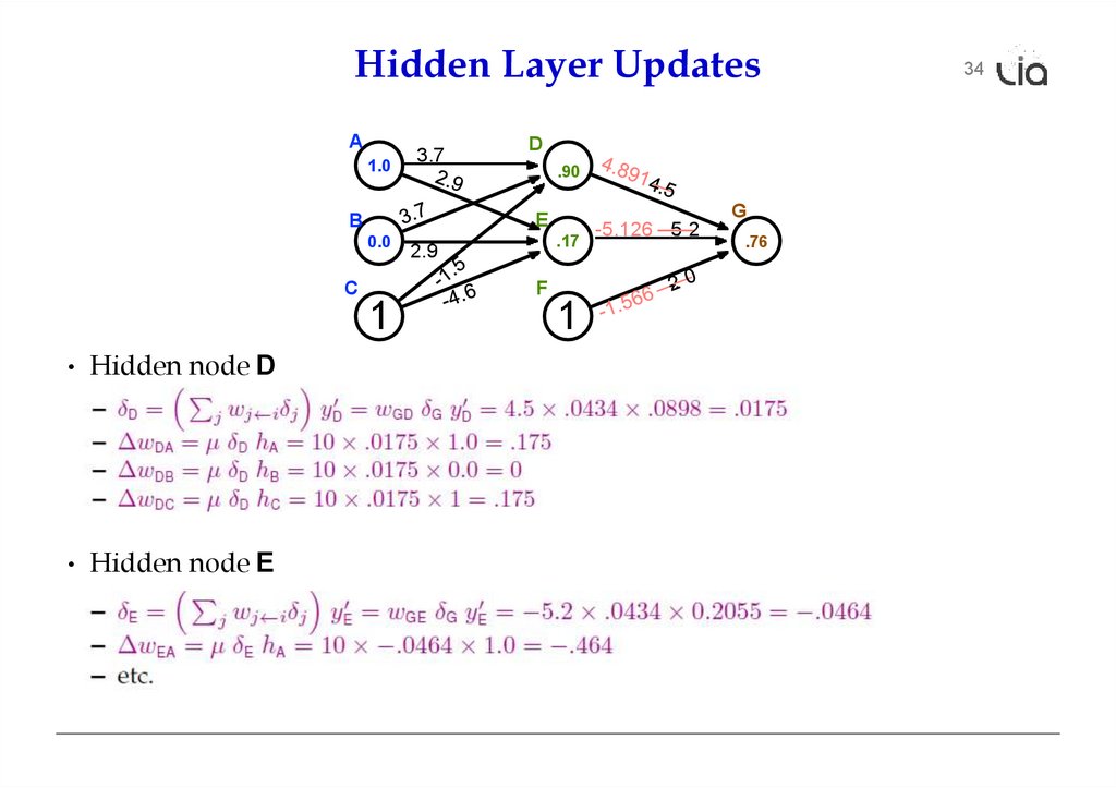
17.

Hidden Layer Updates
A
1.0
3.7
0.0
C
.17
2.9
F
1
• Hidden node E
.90
E
B
• Hidden node D
D
1
-5.126 -—5.—2
G
.76
34

18.

35
some additional aspects

19.

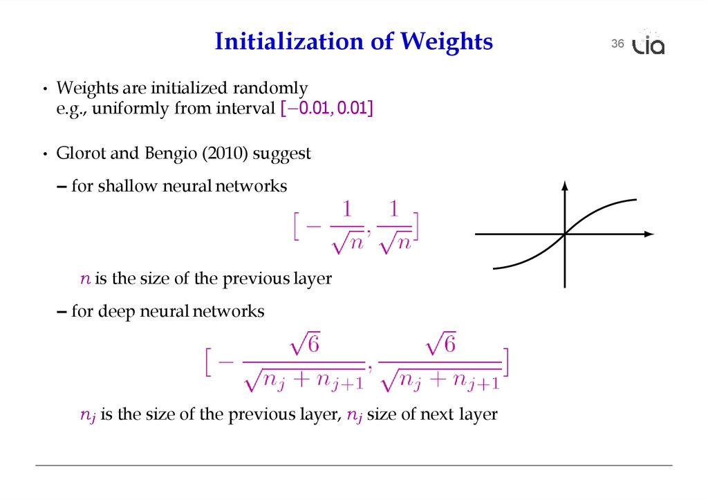
Initialization of Weights
• Weights are initialized randomly
e.g., uniformly from interval [−0.01, 0.01]
• Glorot and Bengio (2010) suggest
– for shallow neural networks
n is the size of the previous layer
– for deep neural networks
n j is the size of the previous layer, n j size of next layer
36

20.

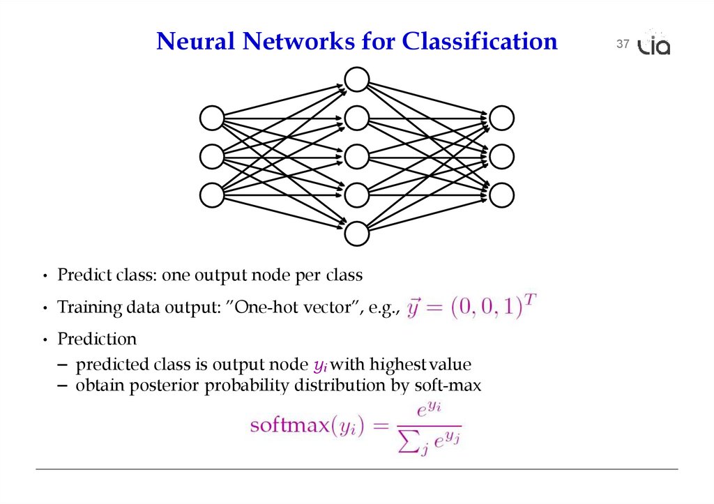
Neural Networks for Classification
• Predict class: one output node per class
• Training data output: ”One-hot vector”, e.g., ˙
• Prediction
– predicted class is output node yi with highest value
– obtain posterior probability distribution by soft-max
37

21.

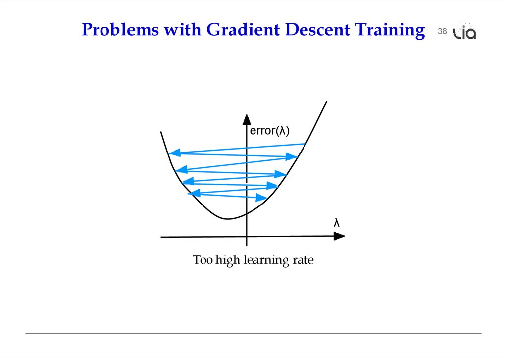
Problems with Gradient Descent Training
error(λ)
λ
Too high learning rate
38

22.

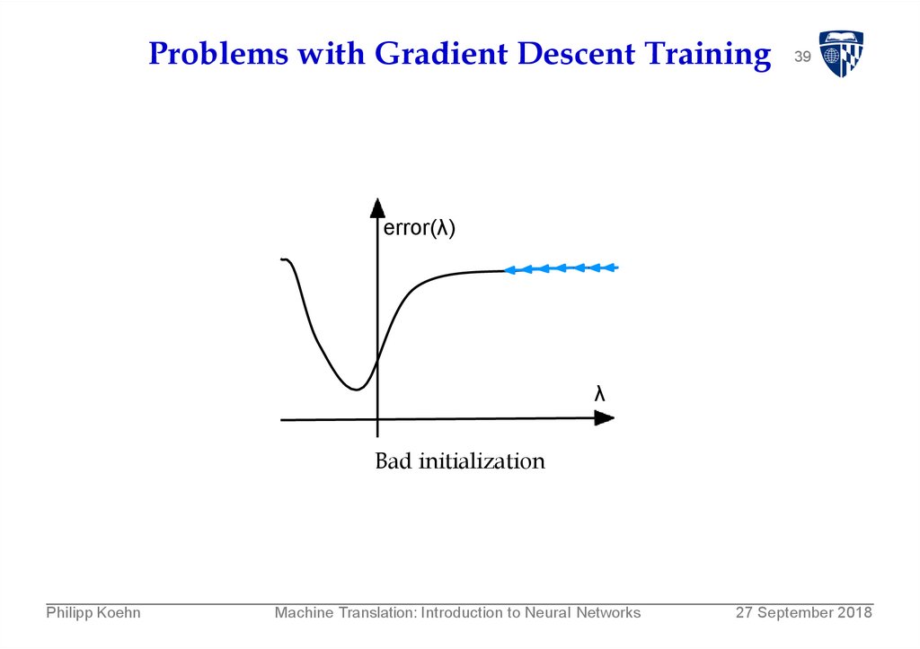
Problems with Gradient Descent Training
39
error(λ)
λ
Bad initialization
Philipp Koehn
Machine Translation: Introduction to Neural Networks
27 September 2018

23.

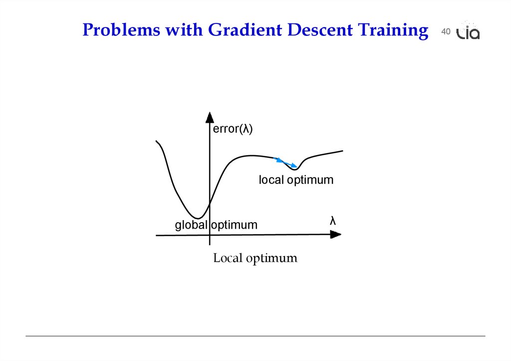
Problems with Gradient Descent Training
error(λ)
local optimum
global optimum
Local optimum
λ
40

24.

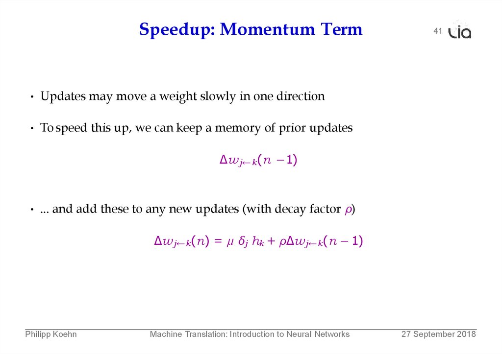
Speedup: Momentum Term
41
• Updates may move a weight slowly in one direction
• To speed this up, we can keep a memory of prior updates
∆wj←k (n −1)
• ... and add these to any new updates (with decay factor ρ)
∆wj←k (n) = µ δj hk + ρ∆wj←k (n − 1)
Philipp Koehn
Machine Translation: Introduction to Neural Networks
27 September 2018

25.

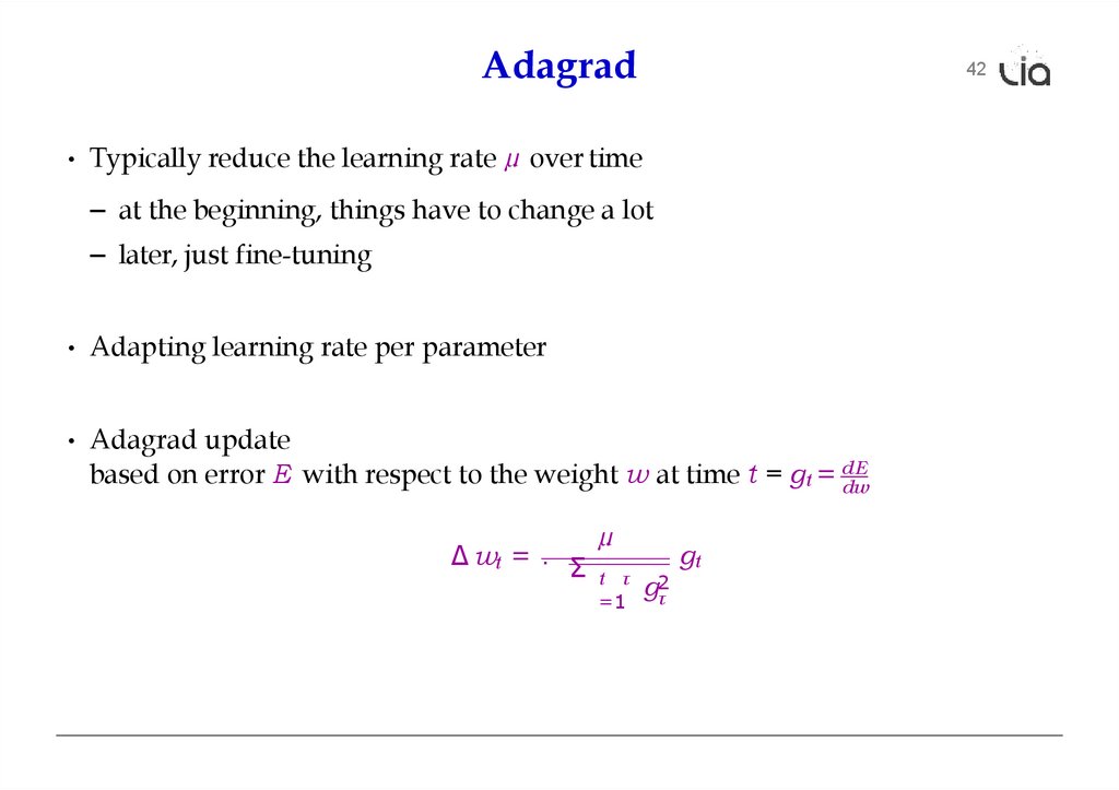
Adagrad
42
• Typically reduce the learning rate µ over time
– at the beginning, things have to change a lot
– later, just fine-tuning
• Adapting learning rate per parameter
• Adagrad update
based on error E with respect to the weight w at time t = gt = dE
dw
∆ wt = . Σ
µ
t τ
=1
gτ2
gt

26.

Dropout
43
• A general problem of machine learning: overfitting to training data
(very good on train, bad on unseen test)
• Solution: regularization, e.g., keeping weights from having extreme values
• Dropout: randomly remove some hidden units during training
– mask: set of hidden units dropped
– randomly generate, say, 10–20 masks
– alternate between the masks during training
• Why does that work?
→ bagging, ensemble, ...

27.

Mini Batches
• Each training example yields a set of weight updates ∆wi .
• Batch up several training examples
– sum up their updates
– apply sum to model
• Mostly done or speed reasons
44

28.

45
computational aspects

29.

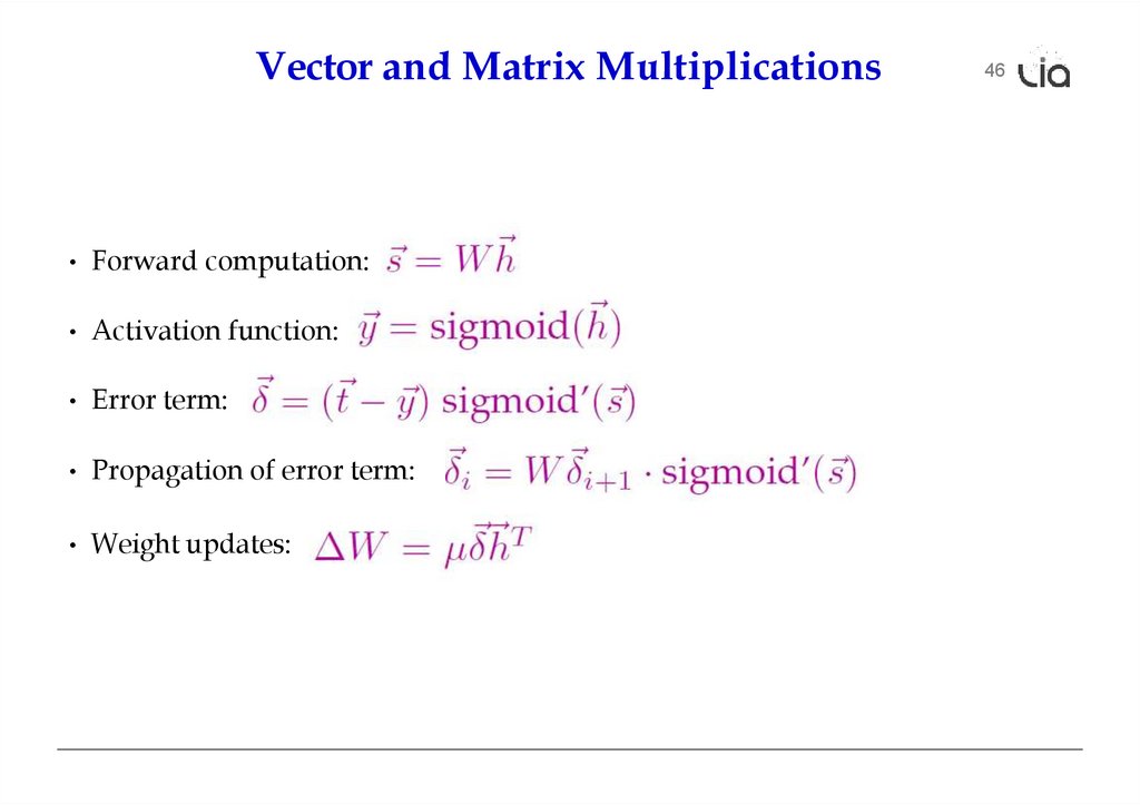
Vector and Matrix Multiplications
• Forward computation:
• Activation function:
• Error term:
• Propagation of error term:
• Weight updates:
46

30.

GPU
• Neural network layers may have, say, 200 nodes
• Computations such as
multiplications
require 200 × 200 = 40, 000
• Graphics Processing Units (GPU) are designed for such computations
– image rendering requires such vector and matrix operations
– massively mulit-core but lean processing units
– example: NVIDIA Tesla K20c GPU provides 2496 thread processors
• Extensions to C to support programming of GPUs, such as CUDA
47

31.

Toolkits
• Theano
• Tensorflow (Google)
• PyTorch (Facebook)
• MXNet (Amazon)
• DyNet
• С (easy api)
48

32.

[email protected]

33.

Next
Tema: Modele secvențiale
Prezentator: Tudor Bumbu