Descriptive statistics

1. Descriptive Statistics

2
Descriptive Statistics
Elementary Statistics
Larson
Larson/Farber Ch 2
Farber
1

2. Section 2.1

Frequency Distributions
and Their Graphs

3. Frequency Distributions

Minutes Spent on the Phone
102
71
103
105
109
124
104
116
97
99
108 86 103
112 118 87
85 122 87
107 67 78
105 99 101
82
95
100
125
92
Make a frequency distribution table with five classes.
Key values:
Larson/Farber Ch 2
Minimum value =
Maximum value =
67
125
3

4. Steps to Construct a Frequency Distribution

1. Choose the number of classes
Should be between 5 and 15. (For this problem use 5)
2. Calculate the Class Width
Find the range = maximum value – minimum. Then divide
this by the number of classes. Finally, round up to a
convenient number. (125 - 67) / 5 = 11.6 Round up to 12
3. Determine Class Limits
The lower class limit is the lowest data value that belongs in a
class and the upper class limit it the highest. Use the minimum
value as the lower class limit in the first class. (67)
4. Mark a tally | in appropriate class for each data value.
After all data values are tallied, count the tallies in each class
for
the class
Larson/Farber
Ch 2 frequencies.
4

5. Construct a Frequency Distribution

Minimum = 67, Maximum = 125
Number of classes = 5
Class width = 12
Class Limits
78
67
Tally
f
3
79
90
5
91
102
8
103
114
9
115
126
5
Do all lower class limits first.
Larson/Farber Ch 2
f =30
5

6. Frequency Histogram

Class
f
Boundaries
67 – 78
3
66.5 - 78.5
79 - 90
5
78.5 - 90.5
91 - 102
8
90.5 - 102.5
Time on Phone
9
9
103 -114
9
102.5 -114.5
8
8
7
115 -126
5
114.5 -126.5
6
f
5
5
5
4
3
3
2
1
0
66.5
78.5
90.5
102.5
114.5
126.5
minutes
Larson/Farber Ch 2
6

7. Frequency Polygon

Class
f
67 - 78
3
79 - 90
5
Time on Phone
9
9
8
8
7
91 - 102
103 -114
115 -126
8
9
5
f
6
5
5
5
4
3
3
2
1
0
72.5
84.5
96.5
108.5
120.5
minutes
Mark the midpoint at the top of each bar. Connect consecutive
midpoints. Extend the frequency polygon to the axis.
Larson/Farber Ch 2
7

8. Other Information

Midpoint: (lower limit + upper limit) / 2
Relative frequency: class frequency/total frequency
Cumulative frequency: Number of values in that class or in lower.
Class
f
Midpoint
Relative
frequency
(67+ 78)/2
3/30
Cumulative
Frequency
67 - 78
3
72.5
0.10
3
79 - 90
5
84.5
0.17
8
91 - 102 8
96.5
0.27
16
103 -114
9
108.5
0.30
25
115 -126
5
120.5
0.17
30
Larson/Farber Ch 2
8

9. Relative Frequency Histogram

Time on Phone
.30
.30
.27
.20
.17
.17
.10
.10
0
66.5
78.5
90.5
102.5 114.5 126.5
minutes
Relative frequency on vertical scale
Larson/Farber Ch 2
9

10. Ogive

Cumulative Frequency
An ogive reports the number of values in the data set that
are less than or equal to the given value, x.
Minutes on Phone
30
30
25
20
16
10
8
3
0
0
66.5
78.5
90.5
102.5
114.5
126.5
minutes
Larson/Farber Ch 2
10

11. Section 2.2

More Graphs and
Displays

12. Stem-and-Leaf Plot

Lowest value is 67 and highest value is 125, so list
stems from 6 to 12.
102
Stem
6 |
7 |
8 |
9 |
10|
11|
12|
Larson/Farber Ch 2
124
108
86
103
82
Leaf
6
2
2
8
3
To see complete
display, go to next
slide.
4
12

13. Stem-and-Leaf Plot

Key: 6 | 7 means 67
6 |7
7 |18
8 |25677
9 |25799
10 | 0 1 2 3 3 4 5 5 7 8 9
11 | 2 6 8
12 | 2 4 5
Larson/Farber Ch 2
13

14. Stem-and-Leaf with two lines per stem

Key: 6 | 7 means 67
1st line digits 0 1 2 3 4
2nd line digits 5 6 7 8 9
1st line digits 0 1 2 3 4
2nd line digits 5 6 7 8 9
Larson/Farber Ch 2
6|7
7|1
7|8
8|2
8|5677
9|2
9|5799
10 | 0 1 2 3 3 4
10 | 5 5 7 8 9
11 | 2
11 | 6 8
12 |2 4
12 | 5
14

15. Dotplot

Phone
66
76
86
96
106
116
126
minutes
Larson/Farber Ch 2
15

16. Pie Chart

Used to describe parts of a whole
Central Angle for each segment
number in category
360o
total number
NASA budget (billions of $) divided
among 3 categories.
Billions of $
Human Space Flight
5.7
Technology
5.9
Mission Support
2.7
Construct a pie chart for the data.
Larson/Farber Ch 2
16

17. Pie Chart

Billions of $
Human Space Flight
Technology
Mission Support
Total
Mission
Support
19%
Technology
41%
Larson/Farber Ch 2
5.7
5.9
2.7
14.3
5.7
360 143
14.3
Human
Space Flight
40%
Degrees
143
149
68
360
5.9
360 149
14.3
NASA Budget
(Billions of $)
17

18. Scatter Plot

x
Absences Grade
x
8
2
5
12
15
9
6
Final
Grade
95
90
85
80
75
70
65
60
55
50
45
40
0
2
4
6
8
10
12
16
14
x
Larson/Farber Ch 2
y
78
92
90
58
43
74
81
Absences
18

19. Section 2.3

Measures of Central
Tendency

20. Measures of Central Tendency

Mean: The sum of all data values divided by
the number of values.
x
x
n
The mean incorporates every value in
the data set.
Median: The point at which an equal number
of values fall above and fall below
Mode: The value with the highest frequency
Larson/Farber Ch 2
20

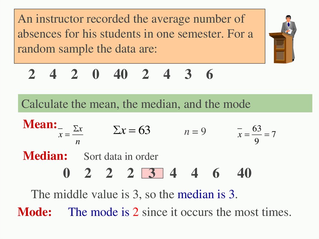
21.

An instructor recorded the average number of
absences for his students in one semester. For a
random sample the data are:
2
4 2 0 40 2 4 3 6
Calculate the mean, the median, and the mode
Mean:
x
Median:
x 63
x
n
n=9
x
63
7
9
Sort data in order
0 2 2
2 3 4 4 6
40
The middle value is 3, so the median is 3.
Mode: The mode is 2 since it occurs the most times.

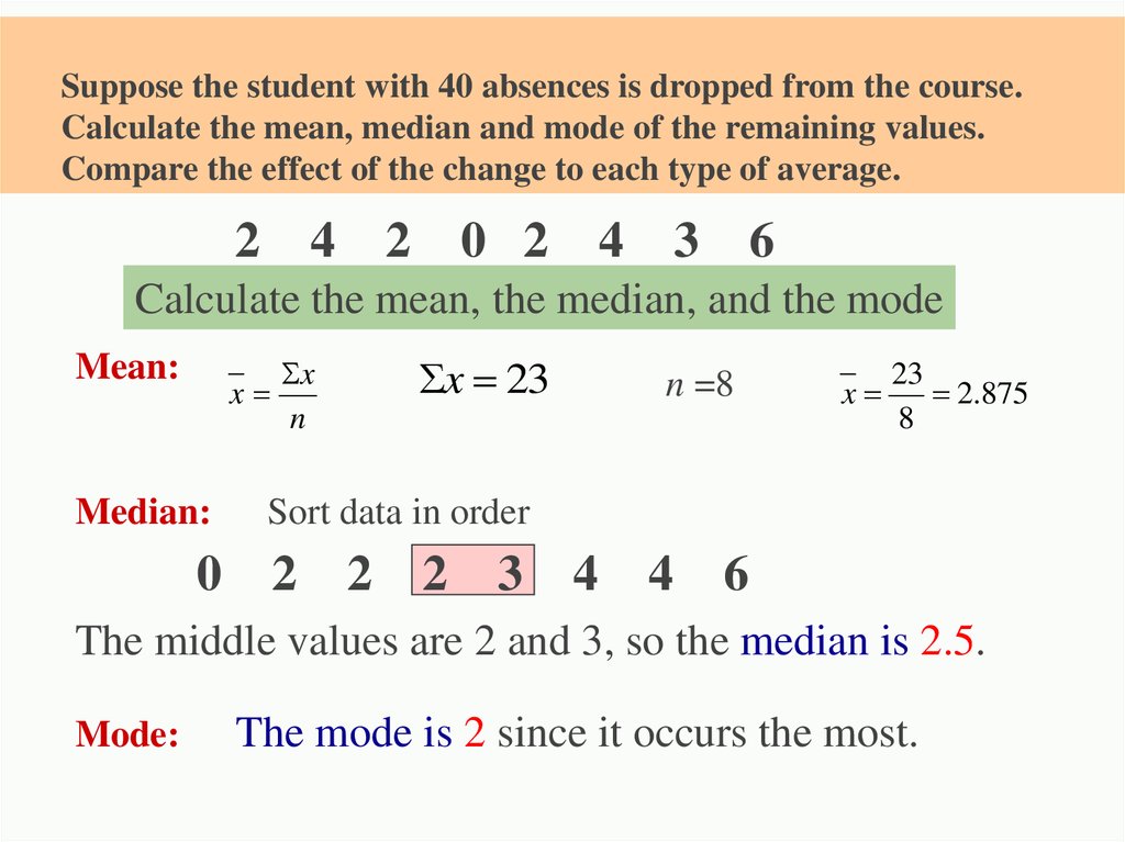
22.

Suppose the student with 40 absences is dropped from the course.
Calculate the mean, median and mode of the remaining values.
Compare the effect of the change to each type of average.
2 4 2 0 2 4 3 6
Calculate the mean, the median, and the mode
Mean:
x
Median:
x
n
x 23
n =8
x
23
2.875
8
Sort data in order
0 2 2 2 3 4 4 6
The middle values are 2 and 3, so the median is 2.5.
Mode:
The mode is 2 since it occurs the most.

23. Shapes of Distributions

Symmetric
1
2
3
4
5
6
7
8
9
10
11
Uniform
12
1
2
3
4
5
6
7
8
9
10
11
12
Mean = Median
Skewed right
1
2
3
4
5
6
7
8
9
10
11
Skewed left
12
Mean is right of median
Mean > Median
Larson/Farber Ch 2
1
2
3
4
5
6
7
8
9
10
11
12
Mean is left of median.
Mean < Median
23

24. Outliers

What happened to our mean, median and mode
when we removed 40 from the data set?
40 is an outlier
An outlier is a value that is much larger or
much smaller than the rest of the values in a
data set.
Outliers have the biggest effect on the mean.
Larson/Farber Ch 2
24

25. Section 2.4

Measures of Variation

26. Measures of Variation

Range = Maximum value - Minimum value
Variance is the sum of the deviations from the
mean divided by n – 1.
Standard deviation is the square root of the
variance.
Larson/Farber Ch 2
26

27. .

Example: A testing lab wishes to test two
experimental brands of outdoor paint to see how long
each will last before fading. The testing lab makes 6
gallons of each paint to test. Since different chemical
agents are added to each group and only six cans are
involved, these two groups constitute two small
populations. The results are shown below.
Brand A: 10, 60, 50, 30, 40, 20
Brand B: 35, 45, 30, 35, 40, 25
Find the mean and range for each brand, then
create a stack plot for each. Compare your
results.
Larson/Farber Ch 2
27

28. Two Data Sets

Closing prices for two stocks were recorded on ten successive
Fridays. Calculate the mean, median and mode for each.
56
56
57
58
61
63
63
Mean = 61.5 67
Median =62 67
Mode= 67
67
Stock A
Larson/Farber Ch 2
33 Stock B
42
48
52
57
67
67
77 Mean = 61.5
82 Median =62
90 Mode= 67
28

29. Measures of Variation

Range = Maximum value - Minimum value
Range for A = 67 - 56 = $11
Range for B = 90 - 33 = $57
The range is easy to compute but only uses 2 numbers
from a data set.
Larson/Farber Ch 2
29

30. To Calculate Variance & Standard Deviation:

To Calculate Variance & Standard Deviation:
1. Find the deviation, the difference between
each data value, x, and the mean, .
2. Square each deviation.
3. Find the sum of all squares from step 2.
4. Divide the result from step 3 by n-1, where
n = the total number of data values in the set.
Larson/Farber Ch 2
30

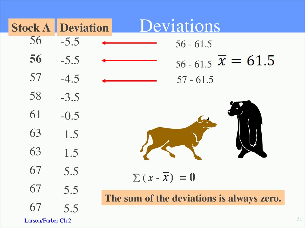
31.

Stock A Deviation
56
-5.5
56
-5.5
57
-4.5
58
-3.5
61
-0.5
63
1.5
63
1.5
67
5.5
67
5.5
67
5.5
Larson/Farber Ch 2
Deviations
56 - 61.5
56 - 61.5
57 - 61.5
(x-
) =0
The sum of the deviations is always zero.
31

32. Variance

Variance: The sum of the squares of the
deviations, divided by n -1.
x
56
56
57
58
61
63
63
67
67
67
x ( x )2
-5.5
-5.5
-4.5
-3.5
-0.5
1.5
1.5
5.5
5.5
5.5
Larson/Farber Ch 2
30.25
30.25
20.25
12.25
0.25
2.25
2.25
30.25
30.25
30.25
188.50
s
2
( x x )
n 1
2
188.50
s
20.94
9
2
Sum of squares
32

33. Standard Deviation

Standard Deviation The square root of the
variance.
The standard deviation is 4.58.
Larson/Farber Ch 2
33

34. Summary

Range = Maximum value - Minimum value
Variance
s
2
( x x )
n 1
2
Standard Deviation
Larson/Farber Ch 2
34

35. Empirical Rule (68-95-99.7%)

Data with symmetric bell-shaped distribution has the
following characteristics.
13.5%
13.5%
68%
2.35%
4
3
2.35%
2
1
0
1
2
3
4
About 68% of the data lies within 1 standard deviation of the mean
About 95% of the data lies within 2 standard deviations of the mean
About 99.7% of the data lies within 3 standard deviations of the mean
Larson/Farber Ch 2
35

36. Using the Empirical Rule

The mean value of homes on a street is $125 thousand with a
standard deviation of $5 thousand. The data set has a bell shaped
distribution. Estimate the percent of homes between $120 and $135
thousand
68%
68%
105
110
115
120
13.5%
68%
125
130
135
140
145
$120 thousand is 1 standard deviation below the mean and $135
thousand is 2 standard deviation above the mean.68% + 13.5% = 81.5%
So, 81.5% have a value between $120 and $135 thousand .
Larson/Farber Ch 2
36

37. Chebychev’s Theorem

For any distribution regardless of shape the
portion of data lying within k standard deviations
(k >1) of the mean is at least 1 - 1/k2.
=6
= 3.84
1
2
3
4
5
6
7
8
9
10
11
12
For k = 2, at least 1-1/4 = 3/4 or 75% of the data
lies within 2 standard deviation of the mean.
For k = 3, at least 1-1/9 = 8/9= 88.9% of the data
lies within 3 standard deviation of the mean.
Larson/Farber Ch 2
37

38. Chebychev’s Theorem

The mean time in a women’s 400-meter dash is
52.4 seconds with a standard deviation of 2.2
sec. Apply Chebychev’s theorem for k = 2.
Mark a number line in
standard deviation units.
2 standard deviations
45.8
48
50.2
52.4
54.6
56.8
59
At least 75% of the women’s 400- meter dash times
will fall between 48 and 56.8 seconds.
Larson/Farber Ch 2
38

39. Section 2.5

Measures of Position

40. Quartiles

3 quartiles Q1, Q2 and Q3 divide the data into 4 equal
parts.
Q2 is the same as the median.
Q1 is the median of the data below Q2
Q3 is the median of the data above Q2
You are managing a store. The average sale for each
of 27 randomly selected days in the last year is given.
Find Q1, Q2 and Q3..
28 43 48 51 43 30 55 44 48 33 45 37 37 42
27 47 42 23 46 39 20 45 38 19 17 35 45
Larson/Farber Ch 2
40

41. Finding Quartiles

The data in ranked order (n = 27) are:
17 19 20 23 27 28 30 33 35 37 37 38 39 42 42
43 43 44 45 45 45 46 47 48 48 51 55 .
Median
Q1=
Q2=
Q3=
Interquartile Range (IQR)= Q3-Q1
IQR =
Larson/Farber Ch 2
41

42. Box and Whisker Plot

A box and whisker plot uses 5 key values to describe a set of data.
Q1, Q2 and Q3, the minimum value and the maximum value.
Q1
Q2 = the median
Q3
Minimum value
Maximum value
30
42
45
17
55
30
42
45
17
15
55
25
35
45
55
Interquartile Range = 45-30=15
Larson/Farber Ch 2
42

43. Percentiles

Percentiles divide the data into 100 parts.
There are 99 percentiles: P1, P2, P3…P99 .
P50 = Q2 = the median
P25 = Q1
P75 = Q3
A 63nd percentile score indicates that score is
greater than or equal to 63% of the scores and
less than or equal to 37% of the scores.
Larson/Farber Ch 2
43

44. Percentiles

30
30
25
20
16
10
8
3
0
0
66.5
78.5
90.5
102.5
114.5
126.5
Cumulative distributions can be used to find percentiles.
114.5 falls on or above 25 of the 30 values.
25/30 = 83.33.
So you can approximate 114 = P83 .
Larson/Farber Ch 2
44

45. Standard Scores

The standard score or z-score, represents the
number of standard deviations that a data value, x
falls from the mean.
value - mean
x
z
standard deviation
The test scores for a civil service exam have a mean
of 152 and standard deviation of 7. Find the standard
z-score for a person with a score of:
(a) 161
Larson/Farber Ch 2
(b) 148
(c) 152
45

46. Calculations of z-scores

(a)
161 152
z
7
z 1.29
(b) 148 152
z
7
z 0.57
(c)
152 152
z
7
z 0
Larson/Farber Ch 2
A value of x =161 is 1.29 standard
deviations above the mean.
A value of x =148 is 0.57 standard
deviations below the mean.
A value of x =152 is equal to the
mean.
46