Introduction to statistics

1. Chapter 1: Introduction to Statistics

1

2.

The structure of presentation:
• A lot of definitions
• Main concepts of statistics
Be ready to learn what does variance, standard deviation
and many other words mean)
• Things that you know
• A little bit of theorems
2

3. Variables

• A variable is a characteristic or condition that can
change or take on different values.
• Most research begins with a general question about the
relationship between two variables for a specific group of
individuals.
3

4. Population

• The entire group of individuals is called the population.
• For example, a researcher may be interested in the
relation between class size (variable 1) and academic
performance (variable 2) for the population of third-grade
children.
4

5. Sample

• Usually populations are so large that a researcher
cannot examine the entire group. Therefore, a sample
is selected to represent the population in a research
study. The goal is to use the results obtained from the
sample to help answer questions about the population.
5

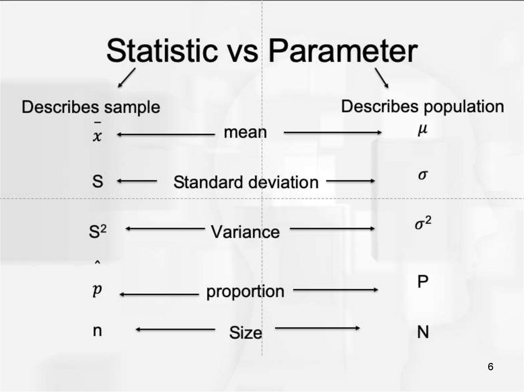
6.

6

7. Types of Variables

Variables can be classified as discrete or continuous.
Discrete variables (such as class size) consist of
indivisible categories (eg: 2 students , cannot be 2.5
students)
• Continuous variables (such as time or weight) are
infinitely divisible into whatever units a researcher may
choose. For example, time can be measured to the
nearest minute, second, half-second, etc.
7

8. Measuring Variables

• To establish relationships between variables,
researchers must observe the variables and record their
observations. This requires that the variables be
measured.
• The process of measuring a variable requires a set of
categories called a scale of measurement and a
process that classifies each individual into one category.
8

9. 4 Types of Measurement Scales

1) A nominal scale is an unordered set of categories identified only by
name (qualitative data).
•Nominal measurements only permit you to determine whether two
individuals are the same or different.
•Order does not matter
Eg: Name, colors, labels, gender, etc.
2) An ordinal scale is an ordered set of categories. Ordinal
measurements tell you the direction of difference between two
individuals. Ranking/ placement
•The order matters
•Difference cannot be measured
Eg: 1st place with score 1.2s, 2nd place with score 2.7s and 3rd place
with score 3.0s
9

10. 4 Types of Measurement Scales

3) An interval scale is an ordered series of equal-sized categories.
Interval measurements identify the direction and magnitude of a
difference. The zero point is located arbitrarily on an interval scale.
• The order matters
• The difference can be measured(except ratios)
• No true “0” starting point
Eg: 25oC, 50oC, 75oC
10

11. 4 Types of Measurement Scales

4) A ratio scale is an interval scale where a value of zero indicates
none of the variable. Ratio measurements identify the direction
and magnitude of differences and allow ratio comparisons of
measurements.
The order matters
Difference measurable(including ratios)
Counts a “0” starting point
Eg: grades in the class, gpa
11

12. Correlational Studies

• The goal of a correlational study is to determine
whether there is a relationship between two variables
and to describe the relationship.
• A correlational study simply observes the two variables
as they exist naturally.
12

13.

14. Experiments

• The goal of an experiment is to demonstrate a causeand-effect relationship between two variables; that is, to
show that changing the value of one variable causes
changes to occur in a second variable.
14

15. Experiments (cont.)

• In an experiment, one variable is manipulated to create
treatment conditions. A second variable is observed and
measured to obtain scores for a group of individuals in
each of the treatment conditions. The measurements
are then compared to see if there are differences
between treatment conditions. All other variables are
controlled to prevent them from influencing the results.
• In an experiment, the manipulated variable is called the
independent variable and the observed variable is the
dependent variable.
• Eg: y=2x+3 ( variable y depends on x)
15

16.

17. Data

• The measurements obtained in a research study are
called the data.
• The goal of statistics is to help researchers organize and
interpret the data.
17

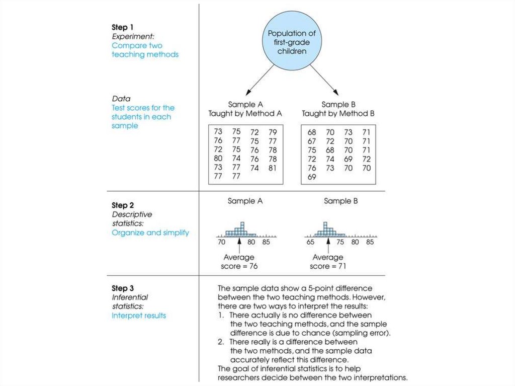
18. Descriptive Statistics

• Descriptive statistics are methods for organizing and
summarizing data.
• For example, tables or graphs are used to organize data,
and descriptive values such as the average score are
used to summarize data.
18

19. Inferential Statistics

• Inferential statistics are methods for using sample data
to make general conclusions (inferences) about
populations.
• Because a sample is typically only a part of the whole
population, sample data provide only limited information
about the population. As a result, sample statistics are
generally imperfect representatives of the corresponding
population parameters.
19

20.

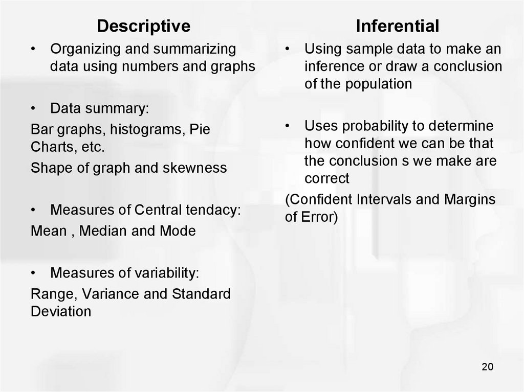
Descriptive
Inferential
• Organizing and summarizing
data using numbers and graphs
• Using sample data to make an
inference or draw a conclusion
of the population
• Data summary:
Bar graphs, histograms, Pie
Charts, etc.
Shape of graph and skewness
• Measures of Central tendacy:
Mean , Median and Mode
• Uses probability to determine
how confident we can be that
the conclusion s we make are
correct
(Confident Intervals and Margins
of Error)
• Measures of variability:
Range, Variance and Standard
Deviation
20

21. Sampling Error

• The discrepancy between a sample statistic and its
population parameter is called sampling error.
• Defining and measuring sampling error is a large part of
inferential statistics.
21

22. Ungrouped Data vs Grouped Data

Ungrouped Data – is a data with an individual value.
Grouped data - have no an individual value.
Says nothing ? Ok, let’s see examples.
22

23. Frequency distribution. Ungrouped Data

• Eg: 2,3,3,5,7,7,7,7,8 ungrouped data
f»
Number
2
3
5
7
8
» 1
» 2
Frequency table
1
4
» 1
total= 9
23

24. Frequency distribution. Grouped data

Eg. In the survey it has been observed that, there are 10
people with a weight between 60-79kg, 13 people between
80-99kg, 2 people between 100-119, and 1 between 120140. Draw a frequency table.
Weight
60-79
80-99
100-119
120-140
f
10
13
2
1
total= 26
24

25. The Mean

• The mean for ungrouped data, also known as the
arithmetic average, is found by adding the values of the
data and dividing by the total number of values. Thus,
25

26.

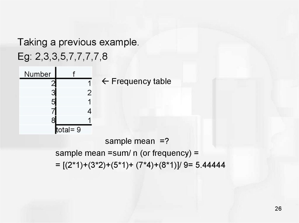
Taking a previous example.
Eg: 2,3,3,5,7,7,7,7,8
Number
f
2
3
5
7
8
»
» 1
» 2
Frequency table
1
4
» 1
total= 9
sample mean =?
sample mean =sum/ n (or frequency) =
= [(2*1)+(3*2)+(5*1)+ (7*4)+(8*1)]/ 9= 5.44444
26

27. The Median

• The median is the middle term in a data set.
• There are two possibilities
• 1) If n is odd, then the median is given by the value of
the middle term in a ranked data.
• 2) If n is even, then the median is given by the average
of the values of the two middle term.
27

28. The Mode

• The value that occurs most often in a data set is called
the mode.
28

29. Measures of dispersion for ungrouped data

• Consider the following 2 examples:
Each of these samples has a mean equal to 67. However, the
dispersion of the observations in the two samples differs
greatly. In the first sample all observations are grouped within
2 units of the mean. Only one observation (67) is closer than
13 units to the mean of the second sample, and some are as
far away as 30 units.
29

30. Measures of dispersion

• The measures that help us to know about the spread of
data set are called the measures of dispersion.
• The measures of central tendency and dispersion taken
together give a better picture of a data set than measure
of central tendency alone.
• Several quantities that are used as measures of
dispersion are the range, the mean absolute
deviation, the variance, and the standard deviation.
30

31. Range

• The range for a set of data is the difference between the
largest and smallest values in the set.
• Range=Largest value-Smallest value
31

32. The mean absolute deviation

• The mean absolute deviation is defined exactly as the
words indicate. The word “deviation” refers to the
deviation of each member from the mean of the
population.
• The term “absolute deviation” means the numerical (i.e.
positive) value of the deviation, and the “mean absolute
deviation” is simply the arithmetic mean of the absolute
deviations.
32

33. Mean Absolute deviation (MAD)

33

34. The variance and the standard deviation

• The average of the squared deviations for a data set
representing a population or sample is given a special
name in statistics. It is called the variance.
• The formula for population variance is
34

35. The variance and the standard deviation

35

36. The variance and the standard deviation

36

37. The variance and the standard deviation

Example: Find the variance and the standard deviation
for the sample of 16, 19, 15, 15, and 14
37

38. Chebyshev’s theorem

38

39. Chebyshev’s theorem

39

40. The interquartile range

40

41. Small revision

41

42.

42

43. Mean for data with multiple-observation values

Mean for data with multipleobservation values
For Population:
Mean:
43

44. Mean for data with multiple-observation values

Mean for data with multipleobservation values
For Sample:
44

45. Mean for data with multiple-observation values

Mean for data with multipleobservation values
Example:
The score for the sample of 25 students on a 5-point quiz
are shown below. Find the mean.
45

46. Median for data with multiple-observation values

Median for data with multipleobservation values
Example:
46

47. Median for data with multiple-observation values

Median for data with multipleobservation values
• The 12th and 13th values fall in class 3. 12th value=3 ; 13th
value=3.
• Therefore, Median (3+3)/2=3
47

48. Mode for data with multiple-observation values

Mode for data with multipleobservation values
The mode is the most frequently occurring value. So it
is 29.
48

49. Variance for data with multiple-observation values

Variance for data with multipleobservation values
49

50. Variance for data with multiple-observation values

Variance for data with multipleobservation values
50

51. A little bit of revision:

Ungrouped Data – is a data with an
individual value.
Grouped data - have no an individual value.
51

52. Frequency distribution. Grouped data

Eg. In the survey it has been observed that, there are 10
people with a weight between 60-79kg, 13 people between
80-99kg, 2 people between 100-119, and 1 between 120140. Draw a frequency table.
Weight
60-79
80-99
100-119
120-140
f
10
13
2
1
total= 26
52

53. Cumulative frequency

For any particular class, the cumulative frequency is
the total number of observations in that and previous
classes.
53

54. Relative frequency

54

55. Histogram

A histogram is a
graph in which
classes are marked
on a horizontal axis
and either the
frequencies are
marked on the
vertical axis. In a
histogram, the bars
are drawn adjacent
to each other.
55

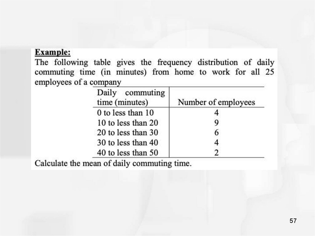
56. Mean for grouped data

56

57.

57

58.

Solution:
58

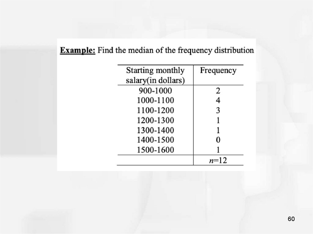
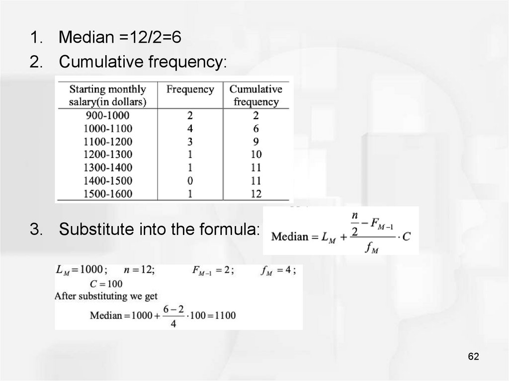
59. The Median for grouped data

59

60.

60

61.

1. Find median
2. Form cumulative frequency
3. Use formula
61

62.

1. Median =12/2=6
2. Cumulative frequency:
3. Substitute into the formula:
62

63. Modal class

The modal class is 2025, since it has the
largest frequency.
Sometimes the
midpoint of the class is
used rather than the
boundaries; hence the
mode could be given
as 22.5.
63

64. Variance and standard deviation for grouped data

64

65. Variance and standard deviation for grouped data

65