


")


")
")


")

")
")


 Математика
Похожие презентации:
")


")


Descriptive Statistics Graphing Techniques
1. Descriptive Statistics Graphing Techniques
2. Points and grades from examination
No. Points Grade No. Points Grade No.Points
Grade
1
15
1
12
12
3
23
15
2
2
17
1
13
16
2
24
9
4
3
19
1
14
13
1
25
17
1
4
10
2
15
7
3
26
16
1
5
2
2
16
15
1
27
13
1
6
14
2
17
20
2
28
6
2
7
5
4
18
16
2
29
16
3
8
17
2
19
14
3
30
18
1
9
11
1
20
3
2
10
16
2
21
15
1
11
10
3
22
12
1
3.
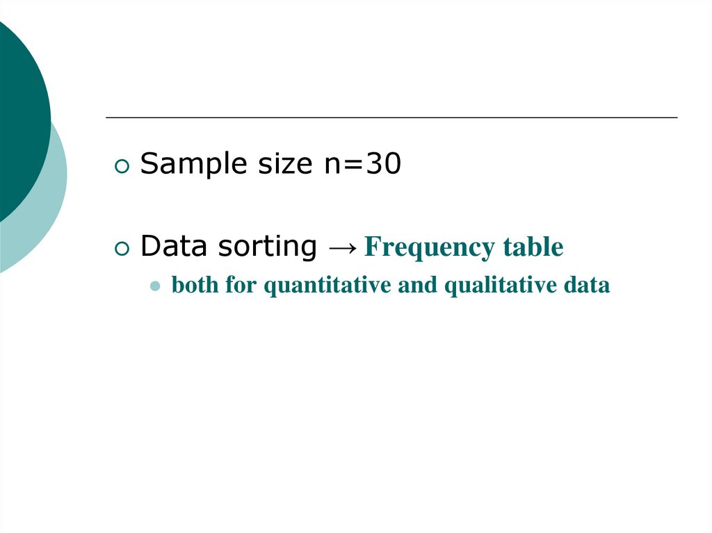
Sample size n=30Data sorting → Frequency table
both for quantitative and qualitative data
4. Exam grade
Exam gradeCumulative Cumulative
Frequency
Percent
12,0
40,0
1
Frequency
12
Percent
40,0
2
11
36,7
23,0
76,7
3
5
16,7
28,0
93,3
4
2
6,7
30,0
100,0
Total
30
100,0
5.
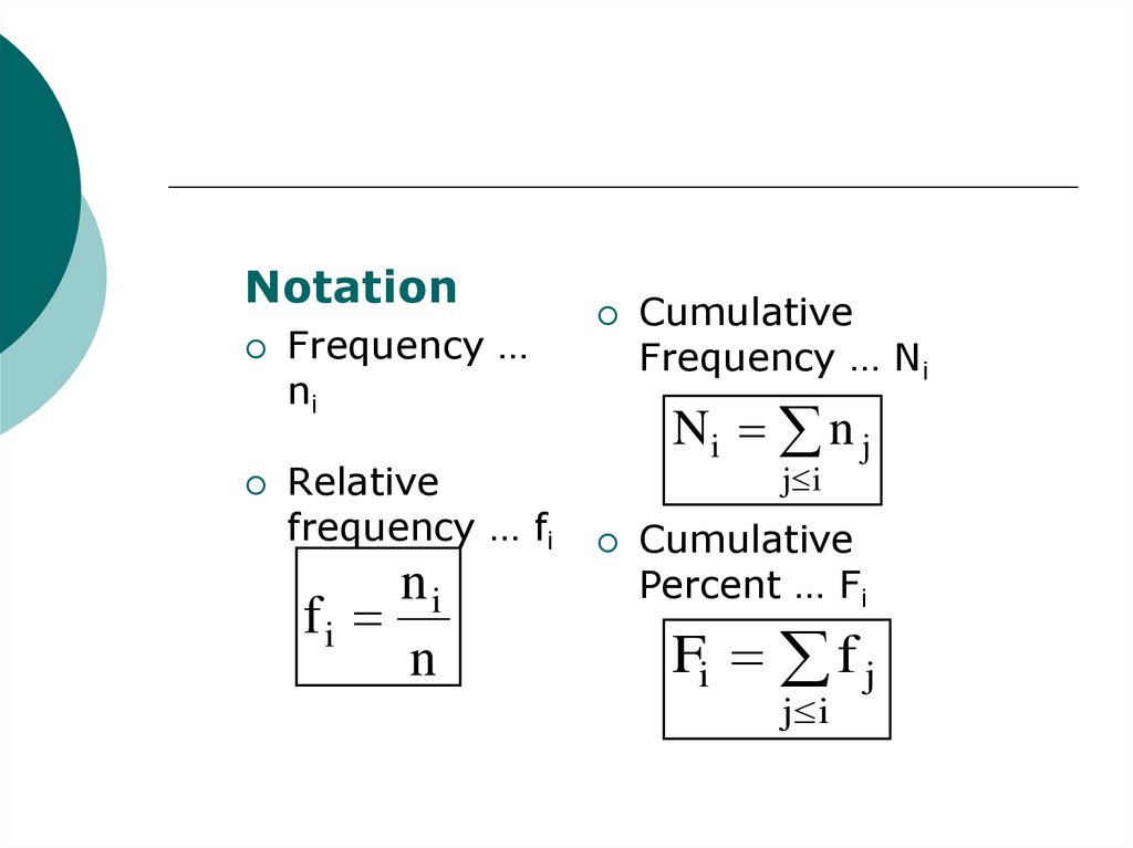
NotationFrequency …
ni
Relative
frequency … fi
ni
fi
n
Cumulative
Frequency … Ni
Ni n j
j i
Cumulative
Percent … Fi
Fi f j
j i
6. Points from class test
Points from class testPoints Frequency Percent Points Frequency Percent
2
1
3,33
13
2
6,67
3
1
3,33
14
2
6,67
5
1
3,33
15
4
13,33
6
1
3,33
16
5
16,67
7
1
3,33
17
3
10,00
9
1
3,33
18
1
3,33
10
2
6,67
19
1
3,33
11
1
3,33
20
1
3,33
12
2
6,67
30
100,00
Total
7.
Quantitative variablesGrouping into class intervals
8. How to select the intervals
Number of intervals → in order todescribe the characteristics of the data
Simple reccommendation
intervals of the same width
k n
k … number of intervals
n … sample size
9. …then
Rh
k
h … width of interval
R … Range=xmax-xmin
k … number of intervals
Our example:
n=30
R=20-2=18
k 30 5,48 6
18
h
3
6
10. Points from class test
Points from class testInterval
5 and
less
Cumulative Cumulative
Frequency
Percent
Frequency
Percent
3
10,0
3
10,0
6-9
3
10,0
6
20,0
10-13
7
23,3
13
43,3
14-17
14
46,7
27
90,0
18 and
more
3
10,0
30
100,0
Total
30
100,0
11. Measures of Central Tendency
Measures that representwith a proper value the tendency of
most data to gather around this
value
Number of different measures of
central tendency
the arithmetic mean
the median
the mode
12. The arithmetic mean
xThe arithmetic mean
Notation
arithmetic mean ……
x
the sum of the values of a variable
divided by the number of scores (by the
sample size)
n
xi
x1 x2 x3 ... xn i 1
x
n
n
13. Properties of the arithmetic mean
1. it is expressed in the same unit of measureas the observed variable
2. it is the point in a distribution of
measurements about which the sum of
deviations are equal to zero
n
( xi x ) 0
i 1
Note: deviation explains the distance and direction from
a reference point – here the arithmetic mean, it is positive
when the value is greater than the mean and negative
when lower than the mean
3. the mean is very sensitive to extreme
values
14. Personal income (thousands CZK)
No.xi
xi x
No.
xi
xi x
1
13,2
-12,62
9
16,4
-9,42
2
13,5
-12,32
10
17,2
-8,62
3
14,0
-11,82
11
19,0
-6,82
4
14,5
-11,32
12
25,8
-0,02
5
14,5
-11,32
13
27,0
1,18
6
15,2
-10,62
14
35,0
9,18
7
15,6
-10,22
15
35,5
9,68
8
16,2
-9,62
16
120,5
94,68
∑
413,1 0,00
n
(x i x) 0
i 1
13,2 ... 120,5 413,1
x
25,82 thousands CZK
16
16
15.
12 of 16 values are below the arithmetic mean,because of the highest value x16=120,5 (directors
income)
personal income is a commonly studied
variable in which other measure of central
tendency is preferred
16. Other measures of central tendency
The median….~
x
The value above and below which one-half of the
frequencies fall
n…odd number
median case number=(n+1)/2
• n…even number
the arithmetic mean of the two middle values
Properties: Insensitive to extreme values
17. Other measures of central tendency
The mode…. x̂The value that occurs with greatest frequency
• for qualitative (nominal and ordinal) and
quantitative discrete data
• from a statistical perspective it is also the
most probable value
18. Personal income (thousands CZK)
n=16… even numberNo.
No.
xi
xi
1
13,2
9
16,4
2
13,5
10
17,2
3
14,0
11
19,0
4
14,5
12
25,8
5
14,5
13
27,0
6
15,2
14
35,0
7
15,6
15
35,5
8
16,2
16
120,5
the median
the mode
19. Personal income (thousands CZK)
n=16… even numberNo.
No.
xi
xi
1
13,2
9
16,4
2
13,5
10
17,2
3
14,0
11
19,0
4
14,5
12
25,8
5
14,5
13
27,0
6
15,2
14
35,0
7
15,6
15
35,5
8
16,2
16
120,5
the median
x 8 x 9 16,2 16,4
~
x
16,3
2
2
the mode
x̂ 14,5
20. Use of mean, median and mode
The arithmetic meanmember of mathematical system in
advanced statistical analysis
preferred measure of central tendency if
the distribution is not skewed
The median
when the distribution is skewed
The mode
whenever a quick, rough estimate of
central tendency is desired
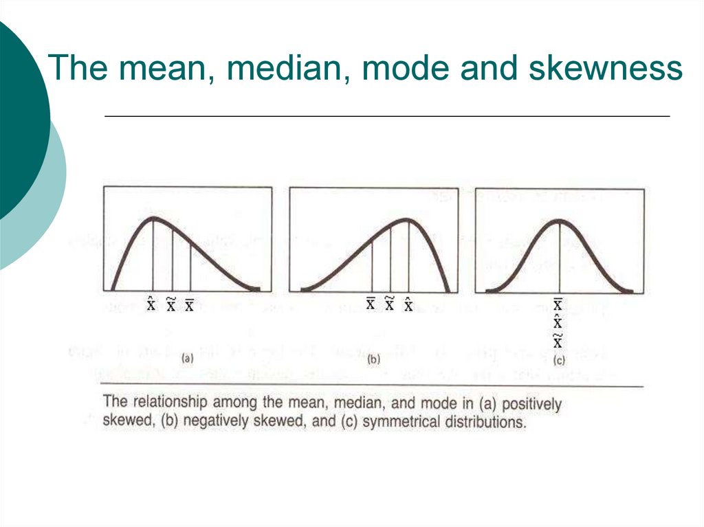
21.
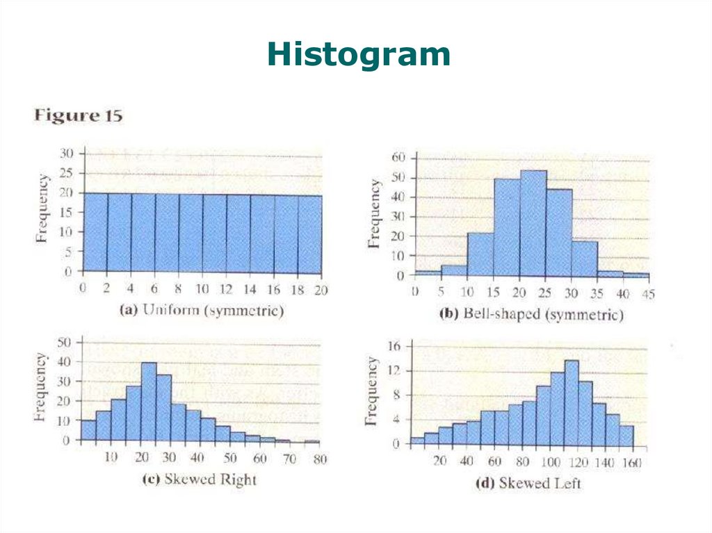
The mean, median, mode and skewness22. Measures of Dispersion
to describe the spread of the data,its variation around a central value
we want to express the distance
along the scale of values
23.
24. The Range….R
it is the distance between thelargest and the smallest value
R=xmax-xmin
it does not explain the variability inside
the range !
very simple and straightforward
measure of dispersion
25. The Variance…s2
it is an average squared deviation ofeach value from the mean
it is the sum of the squared deviations from
the mean divided by n
when computing the variation based on
sample we correct the calculation
n
s
2
(xi x)
i 1
n -1
2
26. Working formulas
For easier computationn
Formula 1
s 2 i 1
n
Formula 2
n
xi x x i
i 1
n -1
2
x
n
x
i
s i 1
2
2
2
n -1
27.
the variance explains boththe variability of the values around the
arithmetic mean
the variability among the values
difficult interpretation
(it is expressed in the squares of the unit of measure)
28. The Standard Deviation…s
it is the square root of variancewhen computing the variation based
on sample
n
s s
2
(xi x)
i 1
n -1
2
29. Properties of the standard deviation
it is expressed in the same unit ofmeasure as the observed variable
the size of the standard deviation is
related to the variability in the values
the more homogeneous values, the smaller
SD
the heterogeneous values, the larger SD
member of mathematical system in
advanced statistical analysis (like the
arthmetic mean)
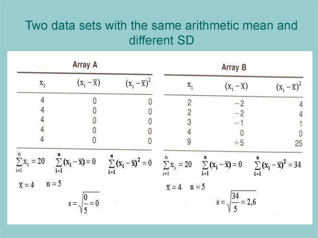
30.
Two data sets with the same arithmetic mean anddifferent SD
31. Example – Personal income (thousands CZK)
No.(x i x)
xi
(x i x) 2
1
13,2
-12,62
159,2644
2
13,5
-12,32
151,7824
…
…
…
…
16
120,5
94,68
8 964,3024
∑
10 370,04
10370,04
s
691,3363
16 1
2
s s 2 691,3363 26,2938 thousands CZK
32. Coefficient of Variation…V
the ratio of the standard deviation tothe mean
s
V
x
often reported as a percentage (%)
by multiplying by 100
33.
it is a relative measure of dispersionused when comparing two data sets
with different units or widely different
means
values higher than 50% indicate
large variability
34. Example – Personal income (thousands CZK)
No.(x i x)
xi
(x i x) 2
1
13,2
-12,62
-159,2644
2
13,5
-12,32
-151,7824
…
…
…
…
16
120,5
94,68
8 964,3024
∑
10 370,04
s 26,2938
x 25,82
s 26,2938
V
1,01835
x
25,82
V 1,01835 *100 101,835%
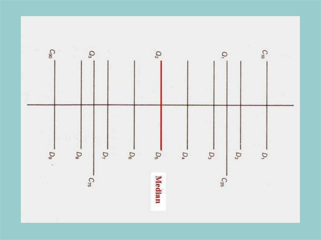
35. Percentiles (Centiles)
value below which a certain percentof observations fall
scale of percentile ranks is
comprised of 100 units
insensitive to extreme values
36. Deciles
divides a distribution into 10 equalparts
there are 9 deciles
D1 – 1st decile
- 10 percent of values fall below it
D9 – 9th decile
- 90 percent of values fall below it
37. Quartiles
divides a distribution into 4 equalparts
Q1 - 25 percent of values fall below it
- 25th centile
Q2 - 50 percent of values fall below it
- 50th centile
Q3 – 75 percent fall below it
- 75th centile
38.
39.
GraphingTechniques
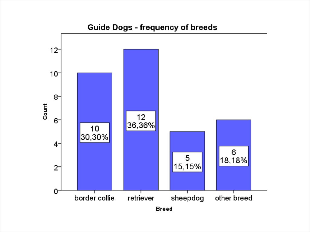
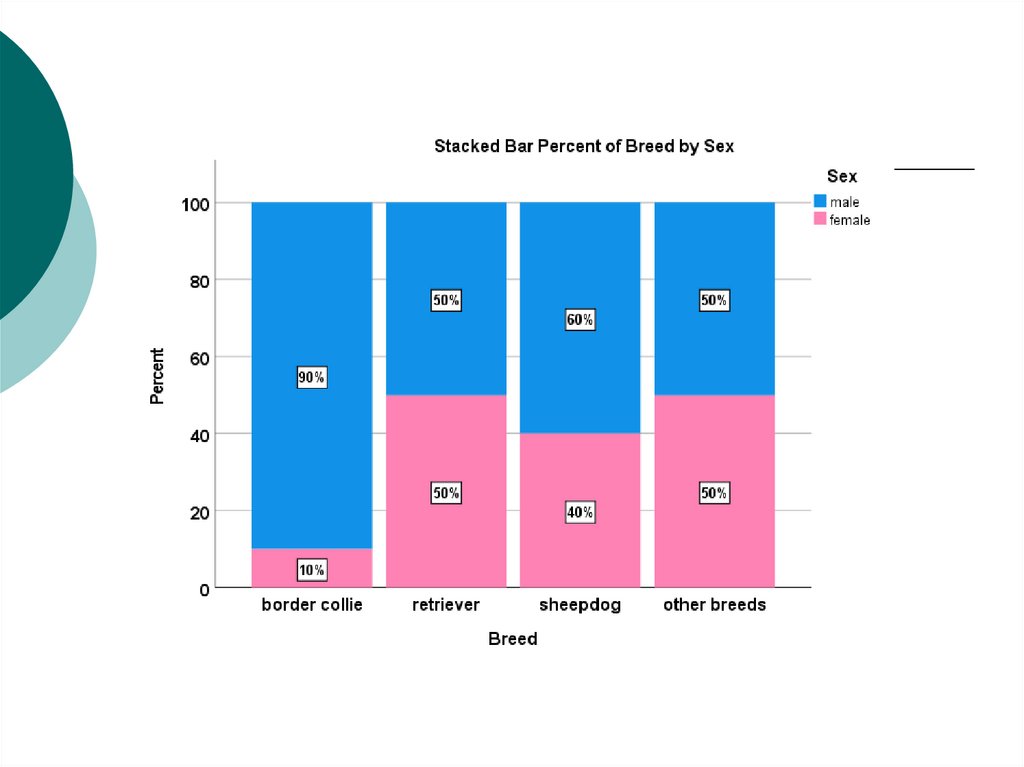
40. Constructing graphs – Bar graph
x – axis: labels of categoriesy – axis: frequency (relative
frequency)
The height of each rectangle is the
category`s frequency or relative
frequency.
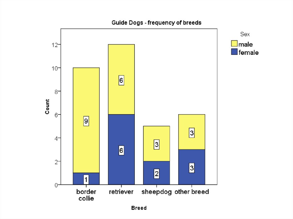
41. Arranging the graph
nominal variables – we canarrange the categories in any
order:alphabetically,
decreasing/increasing order of
frequency
ordinal variables – the categories
should be placed in their naturally
occuring order
42.
43.
44.
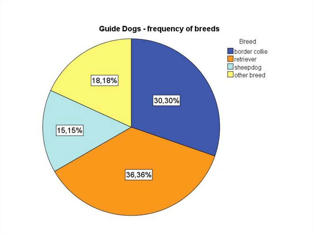
45. Constructing graphs – Pie graph
Pie chart – a circle divided intosectors
each sector represents a category of
data
the area of each sector is proportional
to the frequency of the category
46.
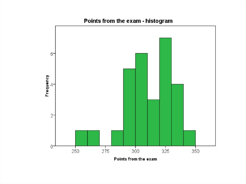
47. Constructing graphs – Histogram
bar graph for quantitative datavalues are grouped into intervals
(classes)
constructed by drawing rectangles
for each class of data
the height of each rectangle is the
frequency of the class
the width of each rectangle is the
same
48.
49.
Histogram50.
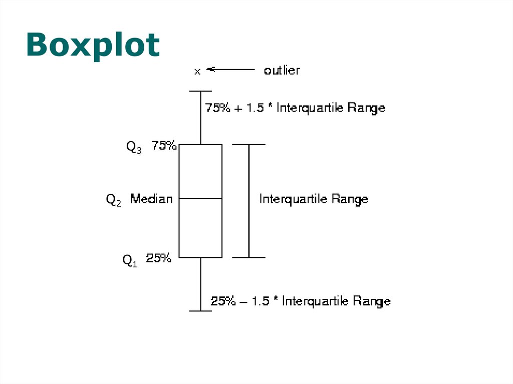
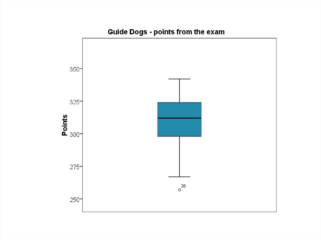
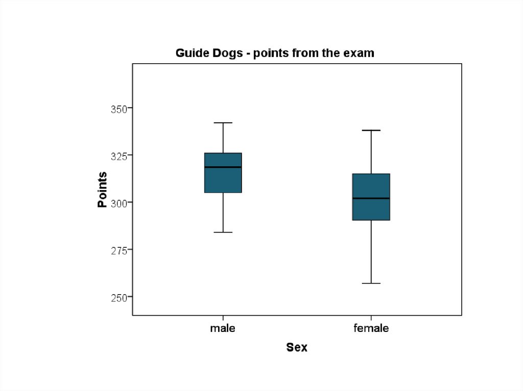
51. Constructing graphs – Boxplot
box-and-whisker diagramfive number summary
52.
BoxplotQ3
Q2
Q1