


")


")


 Английский язык
Похожие презентации:

")


Synchronous Machines Models
1. ECE 576 – Power System Dynamics and Stability
Lecture 10: Synchronous Machines ModelsProf. Tom Overbye
Dept. of Electrical and Computer Engineering
University of Illinois at Urbana-Champaign
overbye@illinois.edu
1
2. Announcements
Homework 2 is due now
Homework 3 is on the website and is due on Feb 27
Read Chapters 6 and then 4
2
3.
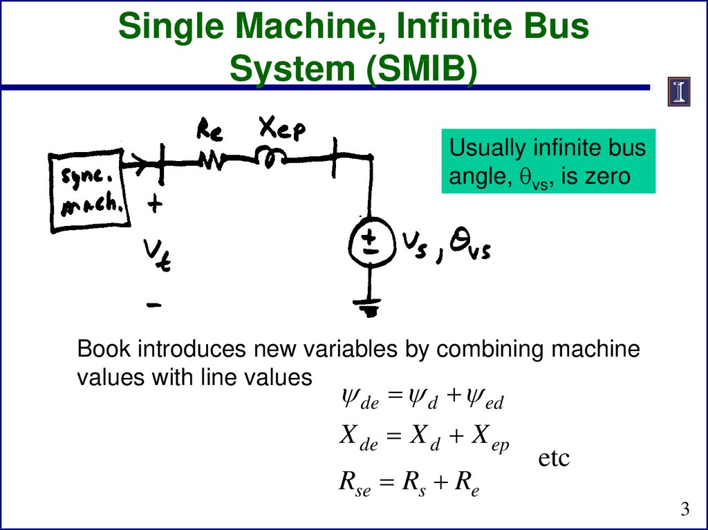
Single Machine, Infinite BusSystem (SMIB)
Usually infinite bus
angle, qvs, is zero
Book introduces new variables by combining machine
values with line values
de d ed
X de X d X ep
Rse Rs Re
etc
3
4.
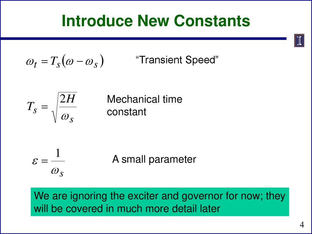
Introduce New Constantst Ts s
Ts
2H
s
1
s
“Transient Speed”
Mechanical time
constant
A small parameter
We are ignoring the exciter and governor for now; they
will be covered in much more detail later
4
5.
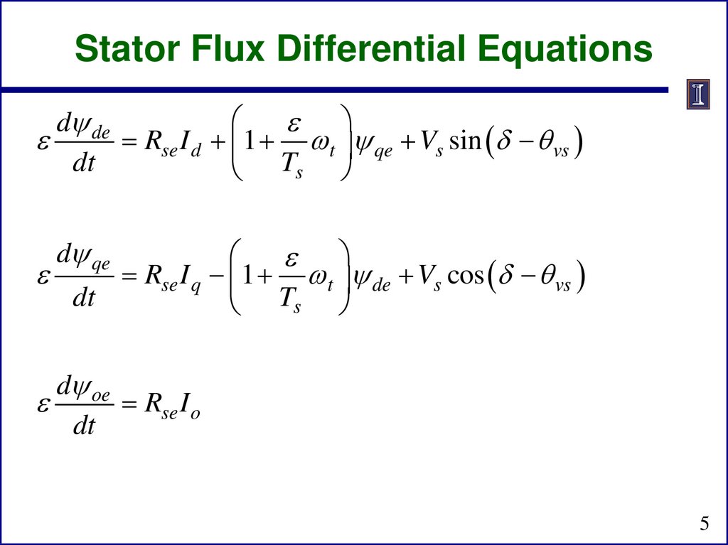
Stator Flux Differential Equationsd de
Rse I d 1 t qe Vs sin q vs
dt
Ts
d qe
Rse I q 1 t de Vs cos q vs
dt
Ts
d oe
Rse I o
dt
5
6.
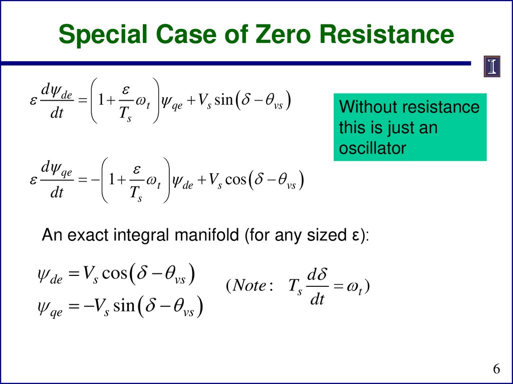
Special Case of Zero Resistanced de
1 t qe Vs sin q vs
dt
Ts
d qe
1 t de Vs cos q vs
dt
Ts
Without resistance
this is just an
oscillator
An exact integral manifold (for any sized ε):
de Vs cos q vs
qe Vs sin q vs
d
( Note : Ts
t )
dt
6
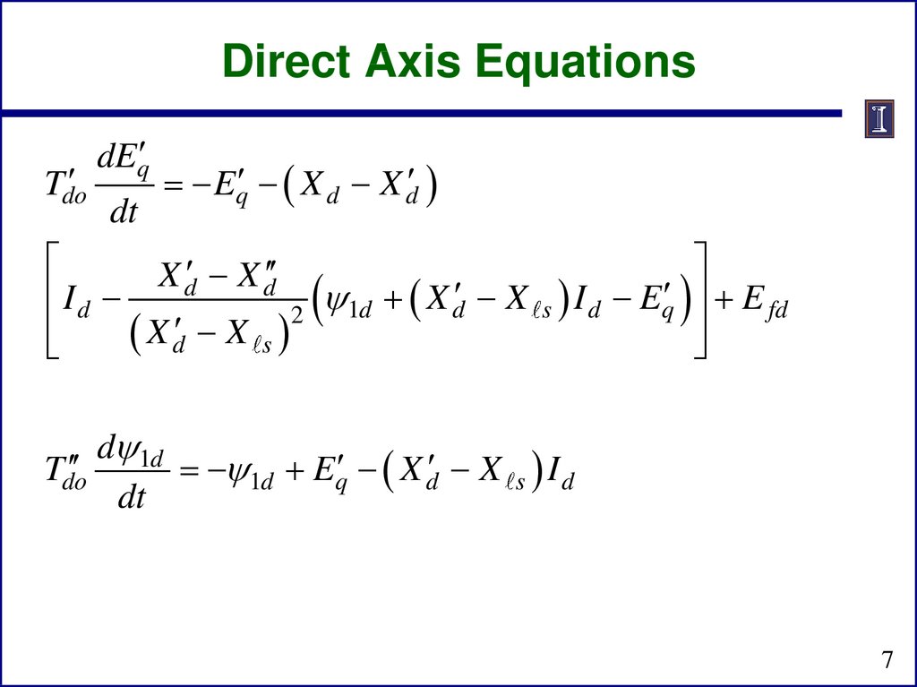
7.
Direct Axis EquationsTdo
dEq
dt
Eq X d X d
X d X d
1d X d X
Id
2
X d X s
s I d Eq E fd
d 1d
Tdo
1d Eq X d X
dt
Id
s
7
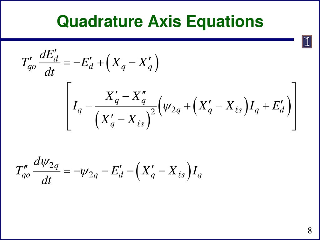
8.
Quadrature Axis EquationsdEd
Tqo
Ed X q X q
dt
X q
X
q
I
2 q X q X
q
2
X s
X
q
Tqo
d 2 q
dt
2 q Ed X q X
s
s
I q Ed
Iq
8
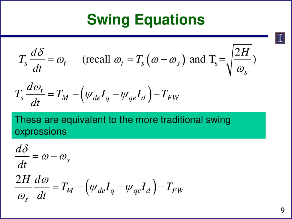
9.
Swing Equationsd
Ts
t
dt
(recall t Ts s and Ts =
2H
s
)
d t
Ts
TM de I q qe I d TFW
dt
These are equivalent to the more traditional swing
expressions
d
s
dt
2 H d
TM de I q qe I d TFW
s dt
9
10.
Stator Flux ExpressionsX d X s
X d X d
I d
de X de
Eq
1d
X d X s
X d X s
X q X s
X q X q
I q
qe X qe
Ed
2q
X q X s X q X s
oe X oe I o
10
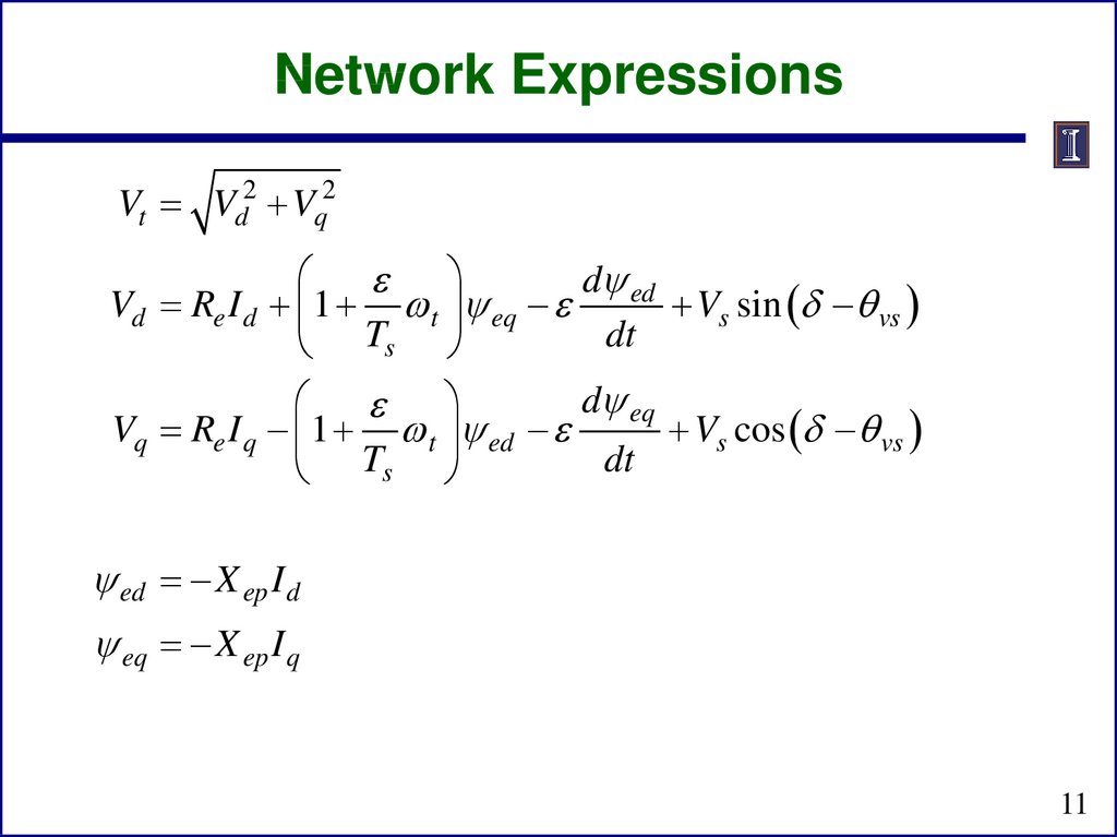
11.
Network ExpressionsVt Vd2 Vq2
d ed
Vd Re I d 1 t eq
Vs sin q vs
dt
Ts
d eq
Vq Re I q 1 t ed
Vs cos q vs
dt
Ts
ed X ep I d
eq X ep I q
11
12.
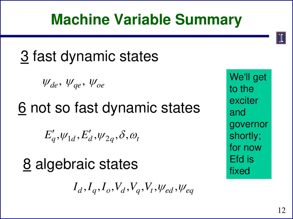
Machine Variable Summary3 fast dynamic states
de , qe , oe
6 not so fast dynamic states
Eq , 1d , Ed , 2 q , , t
8 algebraic states
We'll get
to the
exciter
and
governor
shortly;
for now
Efd is
fixed
I d , I q , I o ,Vd ,Vq ,Vt , ed , eq
12
13. Elimination of Stator Transients
If we assume the stator flux equations are much faster
than the remaining equations, then letting go to zero
creates an integral manifold with
0 Rse I d qe Vs sin q vs
0 Rse I q de Vs cos q vs
0 Rse I o
13
14. Impact on Studies
Image Source: P. Kundur, Power System Stability and Control, EPRI, McGraw-Hill, 199414
15.
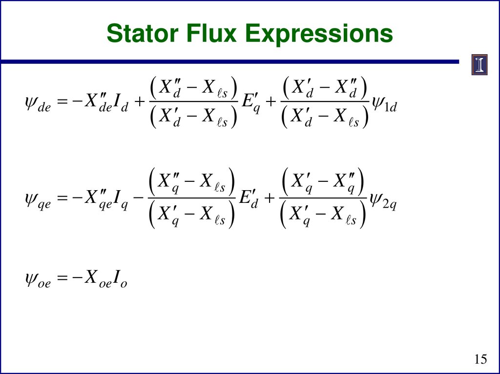
Stator Flux ExpressionsX d X s
X d X d
I d
de X de
Eq
1d
X d X s
X d X s
X q X s
X q X q
I q
qe X qe
Ed
2q
X q X s X q X s
oe X oe I o
15
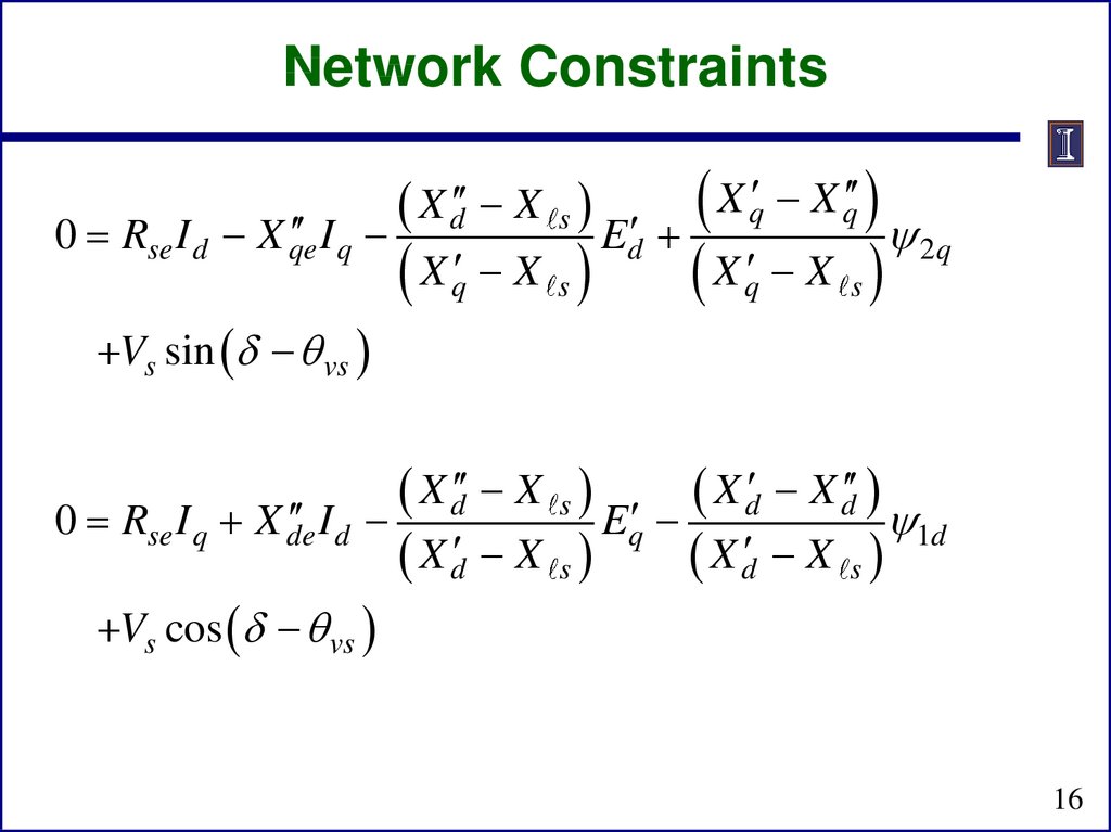
16.
Network ConstraintsI q
0 Rse I d X qe
X q X q
2q
d
X q X s X q X s
X d X s
E
Vs sin q vs
X d X s
X d X d
I d
0 Rse I q X de
Eq
1d
X d X s
X d X s
Vs cos q vs
16
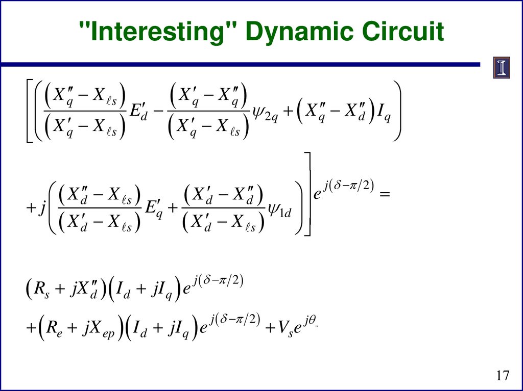
17.
"Interesting" Dynamic CircuitX q X
X q X
E X q X q X X I
d
2q q
d q
X q X s
s
s
j 2
X d X s
e
X d X d
j
Eq
1d
X d X s
X d X s
j 2
Rs jX d I d jI q e
Re jX ep
j 2
I d jI q e
Vs e jq
vs
17
18.
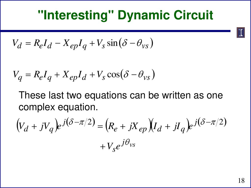
"Interesting" Dynamic CircuitVd Re I d X ep I q Vs sin q vs
Vq Re I q X ep I d Vs cos q vs
These last two equations can be written as one
complex equation.
V jV e j 2 R jX
I jI e j 2
d
q
e
ep
d
q
Vs e jq vs
18
19.
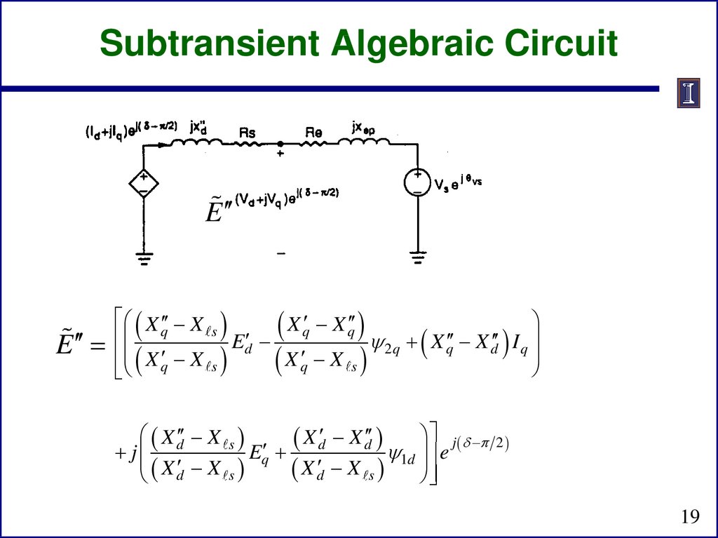
Subtransient Algebraic CircuitE
E
X q X
X q X
E X q X q X X I
d
2q q
d q
X
X
q s
s
s
X d X
j
X d X
E X d X d e j 2
q
1d
X
X
d
s
s
s
19
20.
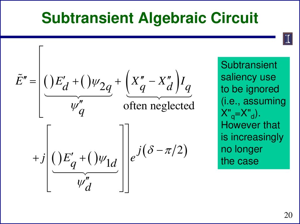
Subtransient Algebraic CircuitE Ed 2q X q X d I q
q
often neglected
j 2
j Eq 1d e
d
Subtransient
saliency use
to be ignored
(i.e., assuming
X"q=X"d).
However that
is increasingly
no longer
the case
20
21. Simplified Machine Models
Often more simplified models were used to represent
synchronous machines
These simplifications are becoming much less common
Next several slides go through how these models can be
simplified, then we'll cover the standard industrial
models
21
22. Two-Axis Model
If we assume the damper winding dynamics are
sufficiently fast, then T"do and T"qo go to zero, so there
is an integral manifold for their dynamic states
1d Eq X q X
I d
2 q Ed X q X s I q
s
22
23. Two-Axis Model
Then
d 1d
Tdo
1d Eq X d X s I d 0
dt
dEq
Tdo
Eq X d X d
dt
X d X d
Id
1d X d X s I d Eq
2
X d X s
dEq
Tdo
Eq X d X d I d E fd
dt
E fd
23
24. Two-Axis Model
And
Tqo
d 2 q
2 q Ed X q X
s
Iq 0
dt
dEd
Tqo
Ed X q X q
dt
I X q X q X X
2q
q
2
q
X q X s
dEd
Tqo
Ed X q X q I q
dt
s
I q Ed
24
25.
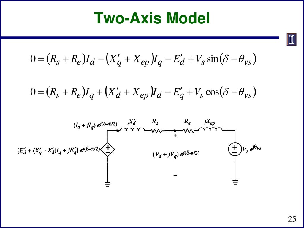
Two-Axis Model0 Rs Re I d X q X ep I q Ed Vs sin q vs
0 Rs Re I q X d X ep I d Eq Vs cos q vs
25
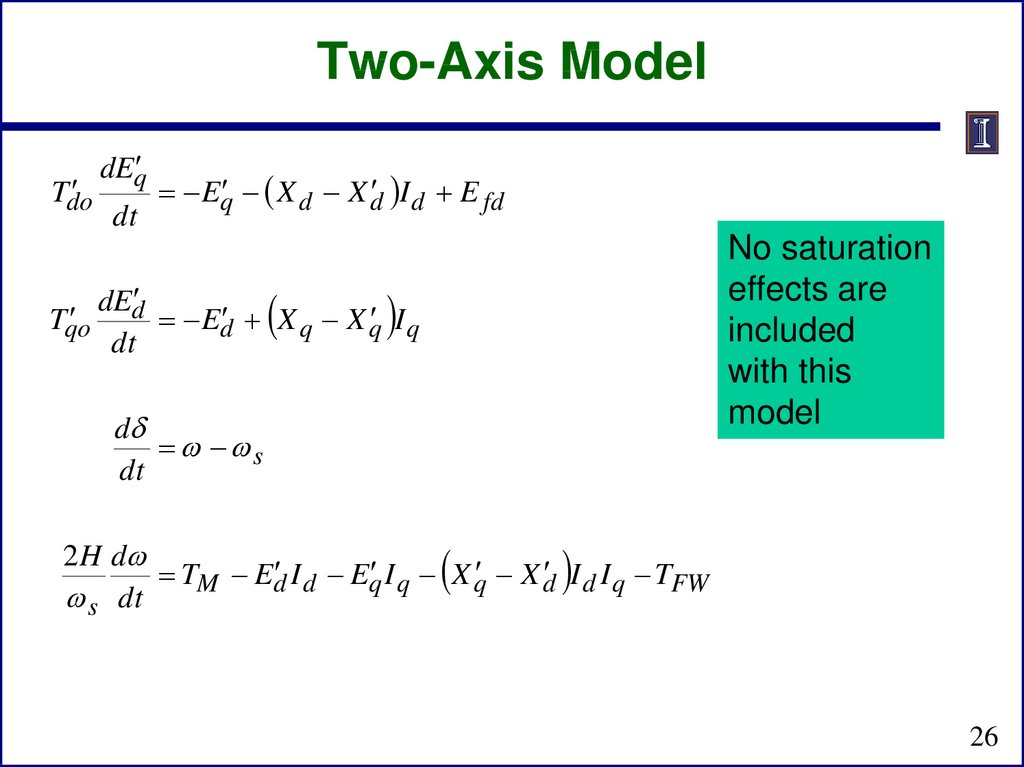
26.
Two-Axis ModelTdo
Tqo
dEq
dt
Eq X d X d I d E fd
dEd
Ed X q X q I q
dt
d
s
dt
No saturation
effects are
included
with this
model
2 H d
TM Ed I d Eq I q X q X d I d I q TFW
s dt
26
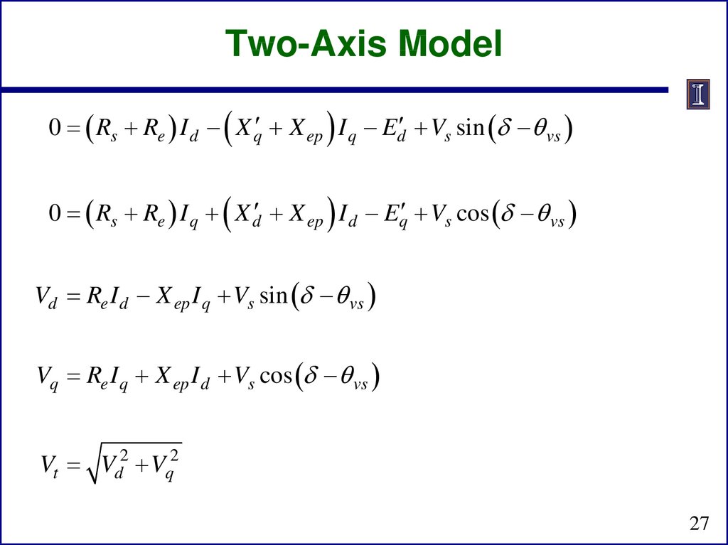
27.
Two-Axis Model0 Rs Re I d X q X ep I q Ed Vs sin q vs
0 Rs Re I q X d X ep I d Eq Vs cos q vs
Vd Re I d X ep I q Vs sin q vs
Vq Re I q X ep I d Vs cos q vs
Vt Vd2 Vq2
27
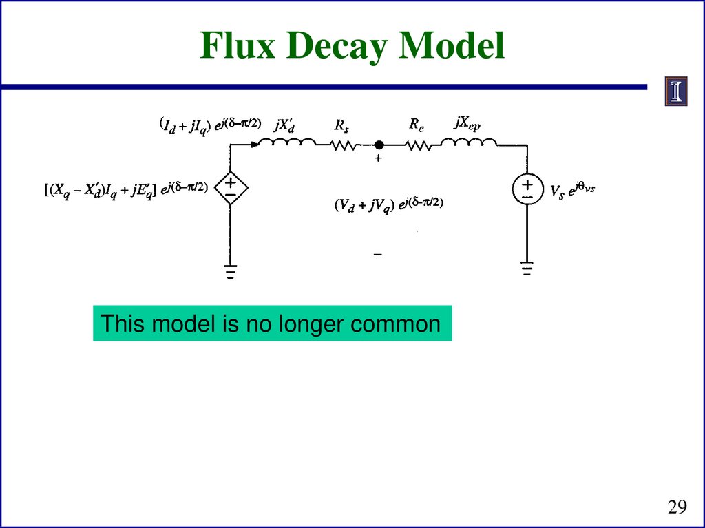
28. Flux Decay Model
If we assume T'qo is sufficiently fast then
dEd
Tqo
Ed X q X q I q 0
dt
dEq
Tdo
Eq X d X d I d E fd
dt
d
s
dt
2H d
TM Ed I d Eq I q X q X d I d I q TFW
s dt
TM X q X q I q I d Eq I q X q X d I d I q TFW
TM Eq I q X q X d I d I q TFW
28
29.
Flux Decay ModelThis model is no longer common
29
30. Classical Model
Has been widely used, but most difficult to justify
Tdo
From flux decay model X q X d
E Eq
0 0
Or go back to the two-axis model and assume
X q X d
E
Tdo
( Eq const
02
Eq
Tqo
Ed const)
02
Ed
0
E
0
1
q
tan
0 2
E
d
30
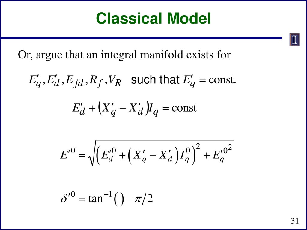
31.
Classical ModelOr, argue that an integral manifold exists for
Eq , Ed , E fd , R f ,VR such that Eq const.
Ed X q X d I q const
E
0
Ed 0
X q
0 2
X d I q
02
Eq
0 tan 1 2
31
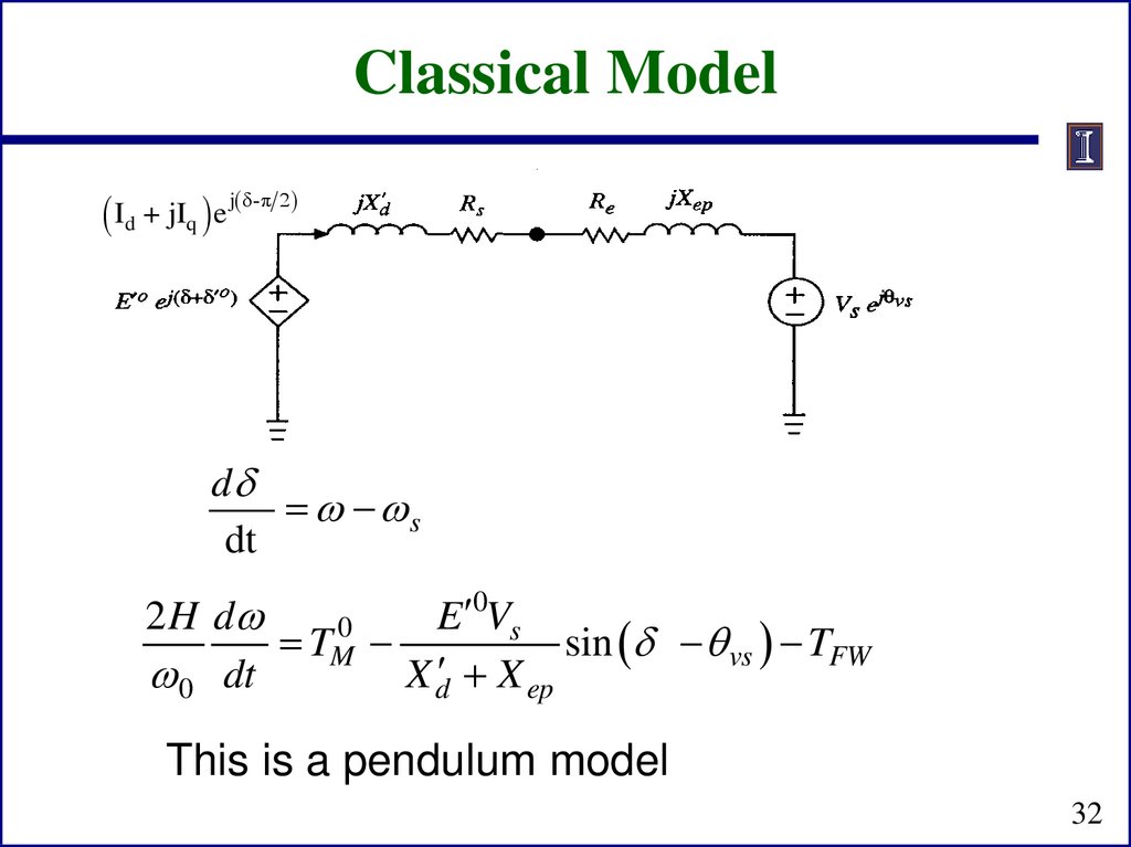
32.
Classical ModelId + jIq e j δ-π 2
d
s
dt
0
2 H d
E
Vs
0
TM
sin q vs TFW
0 dt
X d X ep
This is a pendulum model
32
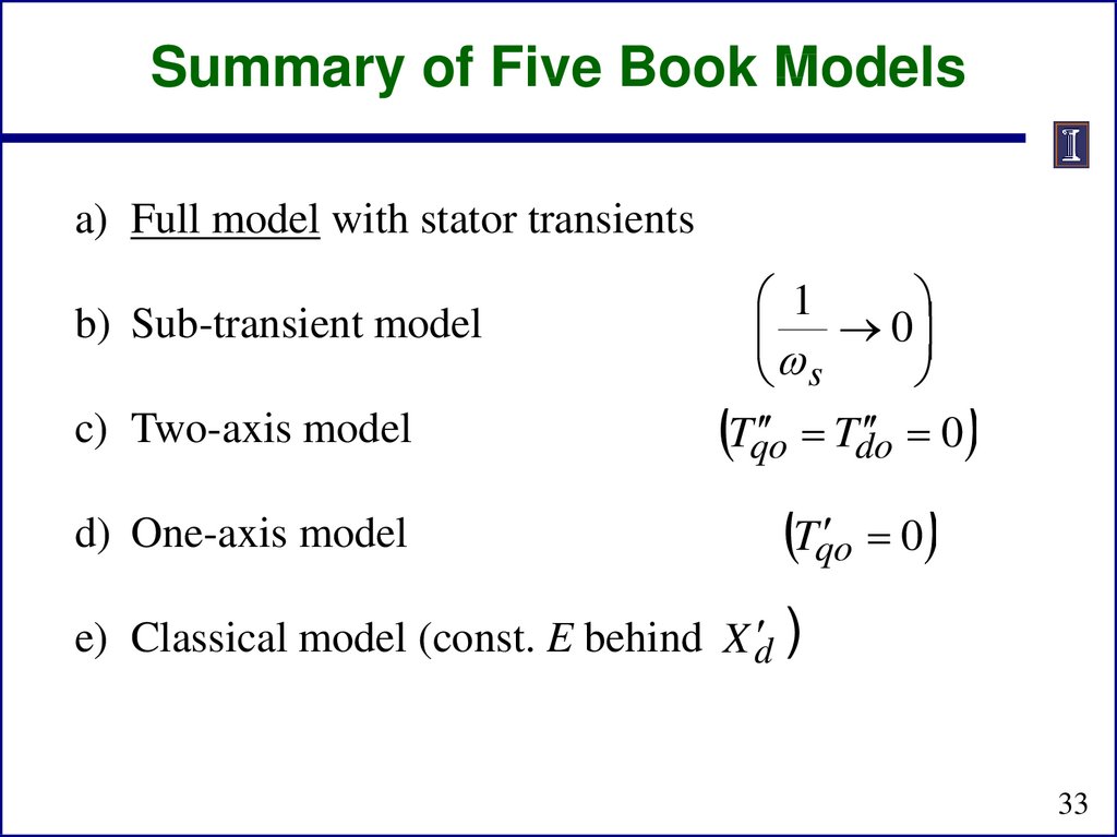
33.
Summary of Five Book Modelsa) Full model with stator transients
c) Two-axis model
1
0
s
Tqo Tdo 0
d) One-axis model
Tqo 0
b) Sub-transient model
e) Classical model (const. E behind X d )
33
34. Damping Torques
Friction and windage
–
Usually small
Stator currents (load)
–
Usually represented in the load models
Damper windings
–
–
Directly included in the detailed machine models
Can be added to classical model as D( - s)
34
35. Industrial Models
There are just a handful of synchronous machine
models used in North America
– GENSAL
• Salient pole model
– GENROU
• Round rotor model that has X"d = X"q
– GENTPF
• Round or salient pole model that allows X"d <> X"q
– GENTPJ
• Just a slight variation on GENTPF
We'll briefly cover each one
35
36. Network Reference Frame
In transient stability the initial generator values are set
from a power flow solution, which has the terminal
voltage and power injection
– Current injection is just conjugate of Power/Voltage
These values are on the network reference frame, with
the angle given by the slack bus angle
V j Vr , j jVi , j In book Vi VDi jVQi
Voltages at bus j converted to d-q reference by
Vd , j sin
V
q , j cos
cos Vr , j
sin Vi , j
Vr , j sin
V
i , j cos
Similar for current; see book 7.24, 7.25
cos Vd , j
sin Vq , j
36
37. Network Reference Frame
Issue of calculating , which is key, will be considered
for each model
Starting point is the per unit stator voltages (3.215 and
3.216 from the book)
Vd q Rs I d
Vq d Rs I q
Equivalently, Vd +jVq Rs I d +jIq q j d
Sometimes the scaling of the flux by the speed is
neglected, but this can have a major impact on the
solution
37
38. Two-Axis Model
We'll start with the PowerWorld two-axis model (twoaxis models are not common commercially, but they
match the book on 6.110 to 6.113
Represented by two algebraic equations and four
differential equations
The bus number subscript
Eq Vq Rs I q X d I d
Ed Vd Rs I d X q I q
dEq
dt
is omitted since it is not used
in commercial block diagrams
1
Eq ( X d X d ) I d E fd ,
Tdo
d
s ,
dt
dEd
1
Ed ( X q X q ) I q
dt
Tqo
2 H d
TM Ed I d Eq I q ( X q X d ) I d I q TFW
s dt
38
39. Two-Axis Model
Value of is determined from (3.229 from book)
E V Rs jX q I
Sign convention on
current is out of the
generator is positive
Once is determined then we can directly solve for E'q
and E'd
39
40. Example (Used for All Models)
Below example will be used with all models. Assume a
100 MVA base, with gen supplying 1.0+j0.3286 power
into infinite bus with unity voltage through network
impedance of j0.22
– Gives current of 1.0-j0.3286 and generator terminal voltage of
1.072+j0.22 = 1.0946 11.59
Bus 4
Bus 1
Bus 2
X12 = 0.20
Infinite Bus
XTR = 0.10
slack
100.00 MW 1.0946 pu
57.24 Mvar 11.59 Deg
1.0463 pu
6.59 Deg
X13 = 0.10
Bus 3
X23 = 0.20
-100.00 MW
-32.86 Mvar
1.0000 pu
0.00 Deg
40
41. Two-Axis Example
For the two-axis model assume H = 3.0 per unitseconds, Rs=0, Xd = 2.1, Xq = 2.0, X'd= 0.3, X'q = 0.5,
T'do = 7.0, T'qo = 0.75 per unit using the 100 MVA base.
Solving we get
E 1.0946 11.59 j 2.0 1.052 18.2 2.814 52.1
52.1
Vd 0.7889 0.6146 1.0723 0.7107
V
0.6146
0.7889
0.220
0.8326
q
I d 0.7889 0.6146 1.000 0.9909
I
q 0.6146 0.7889 0.3287 0.3553
41
42. Two-Axis Example
And
Eq 0.8326 0.3 0.9909 1.1299
Ed 0.7107 (0.5)(0.3553) 0.5330
E fd 1.1299 (2.1 0.3)(0.9909) 2.9135
Saved as case B4_TwoAxis
42
43. Subtransient Models
The two-axis model is a transient model
Essentially all commercial studies now use subtransient
models
First models considered are GENSAL and GENROU,
which require X"d=X"q
This allows the internal, subtransient voltage to be
represented as
E V ( Rs jX ) I
Ed jEq q j d
43
44. Subtransient Models
Usually represented by a Norton Injection with
May also be shown as
Ed jEq q j d
I d jI q
Rs jX
Rs jX
j I d jI q I q jI d
j q j d
Rs jX
j
d
q
Rs jX
In steady-state = 1.0
44
45. GENSAL
The GENSAL model has been widely used to model
salient pole synchronous generators
– In the 2010 WECC cases about 1/3 of machine models were
GENSAL; in 2013 essentially none are, being replaced by
GENTPF or GENTPJ
In salient pole models saturation is only assumed to
affect the d-axis
45
46. GENSAL Block Diagram (PSLF)
A quadratic saturation function is used. Forinitialization it only impacts the Efd value
46
47. GENSAL Initialization
To initialize this model
1.
2.
Use S(1.0) and S(1.2) to solve for the saturation coefficients
Determine the initial value of with
E V Rs jX q I
3.
4.
Transform current into dq reference frame, giving id and iq
Calculate the internal subtransient voltage as
E V ( Rs jX ) I
5.
6.
Convert to dq reference, giving P"d+jP"q= "d+ "q
Determine remaining elements from block diagram by
recognizing in steady-state input to integrators must be zero
47
48. GENSAL Example
Assume same system as before, but with the generator
parameters as H=3.0, D=0, Ra = 0.01, Xd = 1.1, Xq =
0.82, X'd = 0.5, X"d=X"q=0.28, Xl = 0.13, T'do = 8.2, T"do
= 0.073, T"qo =0.07, S(1.0) = 0.05, and S(1.2) = 0.2.
Same terminal conditions as before
Current of 1.0-j0.3286 and generator terminal voltage of
1.072+j0.22 = 1.0946 11.59
Use same equation to get initial
E V Rs jX q I
1.072 j 0.22 (0.01 j 0.82)(1.0 j 0.3286)
1.35 j1.037 1.70 37.5
48
49. GENSAL Example
Then
I d sin cos I r
I
I
cos
sin
i
q
0.609 0.793 1.0 0.869
0.793
0.609
0.3286
0.593
And
V ( Rs jX ) I
1.072 j 0.22 (0.01 j 0.28)(1.0 j 0.3286)
1.174 j 0.497
49
50. GENSAL Example
Giving the initial fluxes (with = 1.0)
q 0.609 0.793 1.174 0.321
0.793 0.609 0.497 1.233
d
To get the remaining variables set the differential
equations equal to zero, e.g.,
q X q X q I q 0.82 0.28 0.593 0.321
Eq 1.425, d 1.104
Solving the d-axis requires solving two linear
equations for two unknowns
50
51. GENSAL Example
Once E'q has been determined, the initial field current
(and hence field voltage) are easily determined by
recognizing in steady-state the E'q is zero
E fd Eq 1 Sat ( Eq ) X d X d I D
Saturation
coefficients
2
1.425 1 B Eq A 1.1 0.5 (0.869) were
determined
2
1.425 1 1.25 1.425 0.8 0.521 2.64 from the two
initial values
Saved as case B4_GENSAL
51