Похожие презентации:
Introduction to normal distributions
1. Section 6-1
Introduction to Normal Distributions© 2012 Pearson Education, Inc. All rights reserved.
1 of 105
2. Section 6-1 Objectives
• Interpret graphs of normal probability distributions• Find areas under the standard normal curve
© 2012 Pearson Education, Inc. All rights reserved.
2 of 105
3. Properties of Normal Distributions
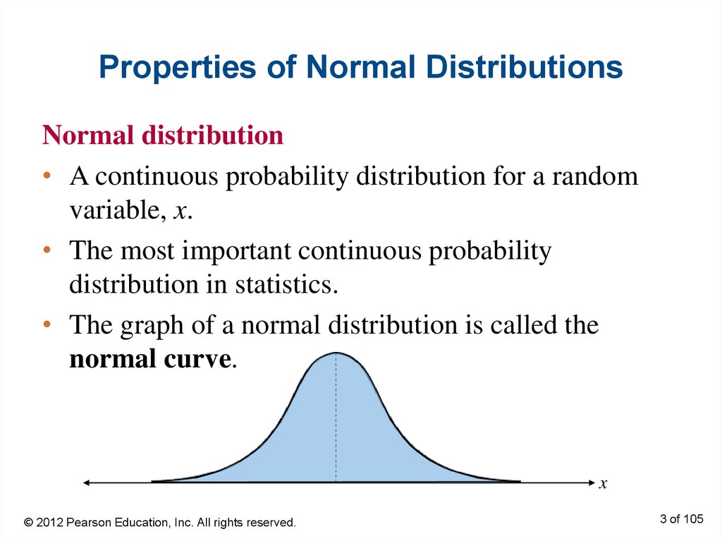
Normal distribution• A continuous probability distribution for a random
variable, x.
• The most important continuous probability
distribution in statistics.
• The graph of a normal distribution is called the
normal curve.
x
© 2012 Pearson Education, Inc. All rights reserved.
3 of 105
4. Properties of Normal Distributions
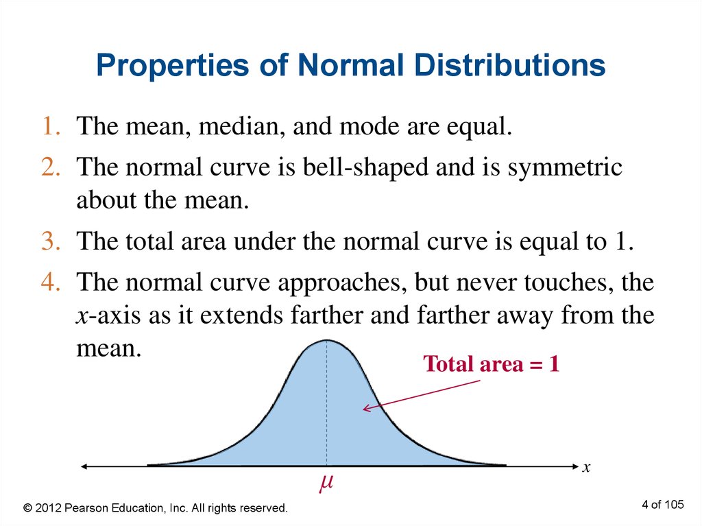
1. The mean, median, and mode are equal.2. The normal curve is bell-shaped and is symmetric
about the mean.
3. The total area under the normal curve is equal to 1.
4. The normal curve approaches, but never touches, the
x-axis as it extends farther and farther away from the
mean.
Total area = 1
μ
© 2012 Pearson Education, Inc. All rights reserved.
x
4 of 105
5. Properties of Normal Distributions
5. Between μ – σ and μ + σ (in the center of the curve),the graph curves downward. The graph curves
upward to the left of μ – σ and to the right of μ + σ.
The points at which the curve changes from curving
upward to curving downward are called the
inflection points.
μ – 3σ
μ – 2σ
μ–σ
© 2012 Pearson Education, Inc. All rights reserved.
μ
μ+σ
μ + 2σ
μ + 3σ
5 of 105
6. Means and Standard Deviations
• A normal distribution can have any mean and anypositive standard deviation.
• The mean gives the location of the line of symmetry.
• The standard deviation describes the spread of the
data.
μ = 3.5
σ = 1.5
© 2012 Pearson Education, Inc. All rights reserved.
μ = 3.5
σ = 0.7
μ = 1.5
σ = 0.7
6 of 105
7. Example: Understanding Mean and Standard Deviation
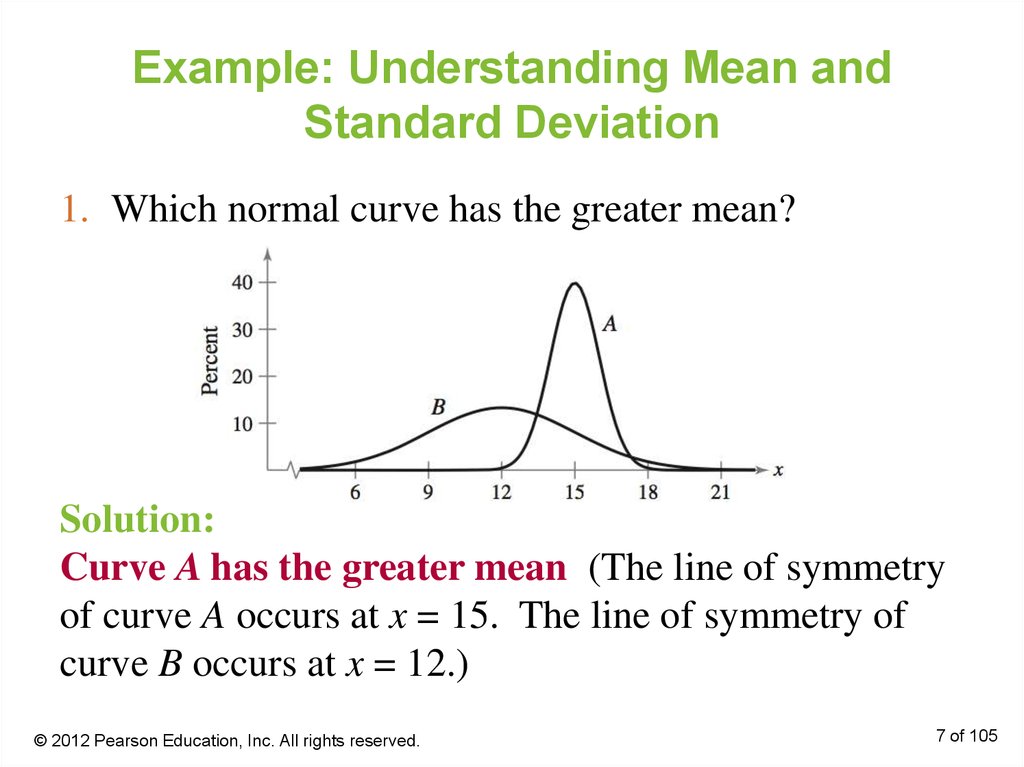
1. Which normal curve has the greater mean?Solution:
Curve A has the greater mean (The line of symmetry
of curve A occurs at x = 15. The line of symmetry of
curve B occurs at x = 12.)
© 2012 Pearson Education, Inc. All rights reserved.
7 of 105
8. Example: Understanding Mean and Standard Deviation
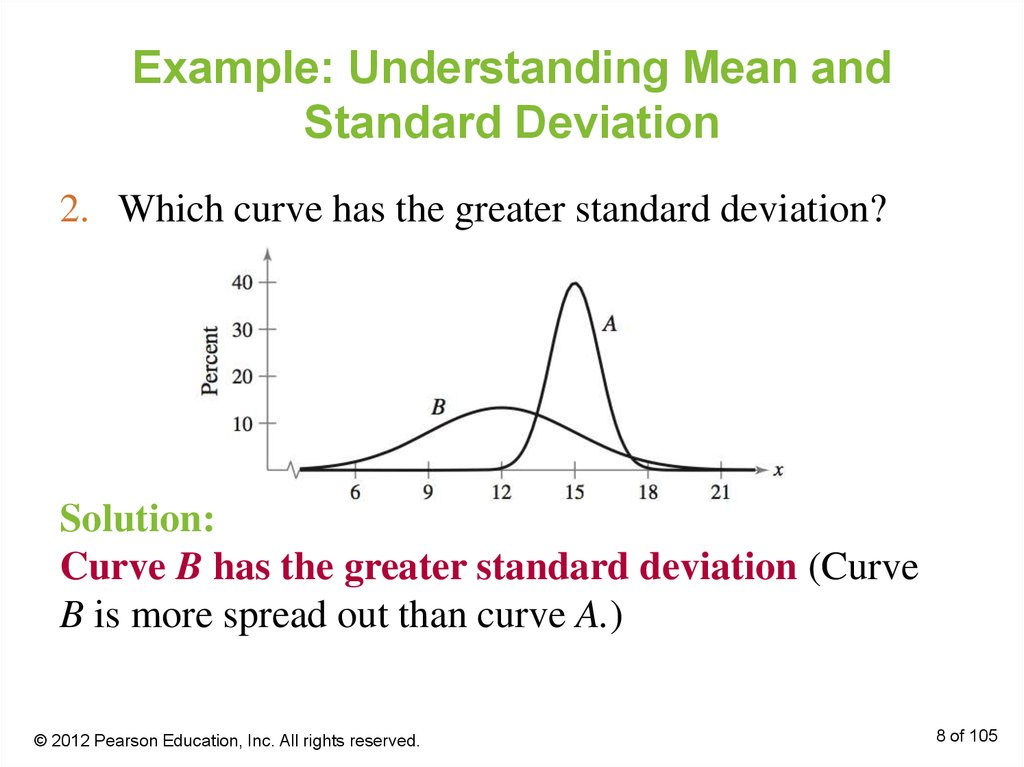
2. Which curve has the greater standard deviation?Solution:
Curve B has the greater standard deviation (Curve
B is more spread out than curve A.)
© 2012 Pearson Education, Inc. All rights reserved.
8 of 105
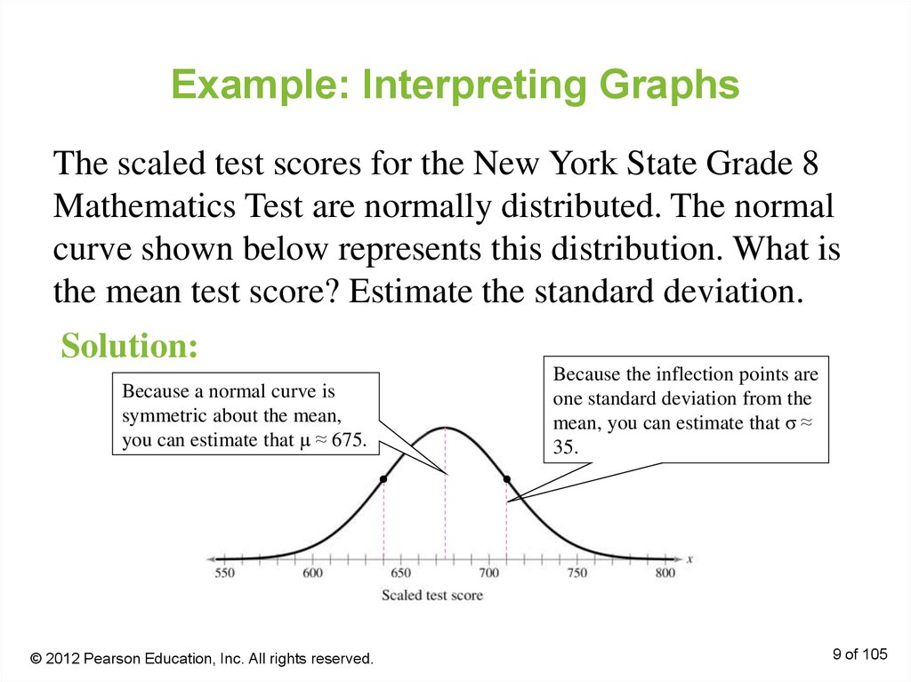
9. Example: Interpreting Graphs
The scaled test scores for the New York State Grade 8Mathematics Test are normally distributed. The normal
curve shown below represents this distribution. What is
the mean test score? Estimate the standard deviation.
Solution:
Because a normal curve is
symmetric about the mean,
you can estimate that μ ≈ 675.
© 2012 Pearson Education, Inc. All rights reserved.
Because the inflection points are
one standard deviation from the
mean, you can estimate that σ ≈
35.
9 of 105
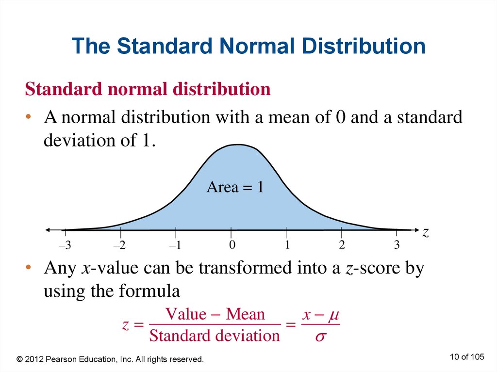
10. The Standard Normal Distribution
Standard normal distribution• A normal distribution with a mean of 0 and a standard
deviation of 1.
Area = 1
–3
–2
–1
z
0
1
2
3
• Any x-value can be transformed into a z-score by
using the formula
Value Mean
x
z
Standard deviation
© 2012 Pearson Education, Inc. All rights reserved.
10 of 105
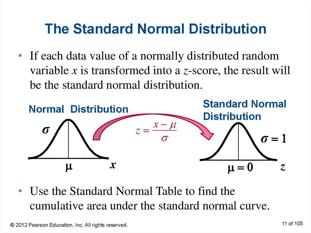
11. The Standard Normal Distribution
• If each data value of a normally distributed randomvariable x is transformed into a z-score, the result will
be the standard normal distribution.
Normal Distribution
σ
z
x
x
Standard Normal
Distribution
σ 1
0
z
• Use the Standard Normal Table to find the
cumulative area under the standard normal curve.
© 2012 Pearson Education, Inc. All rights reserved.
11 of 105
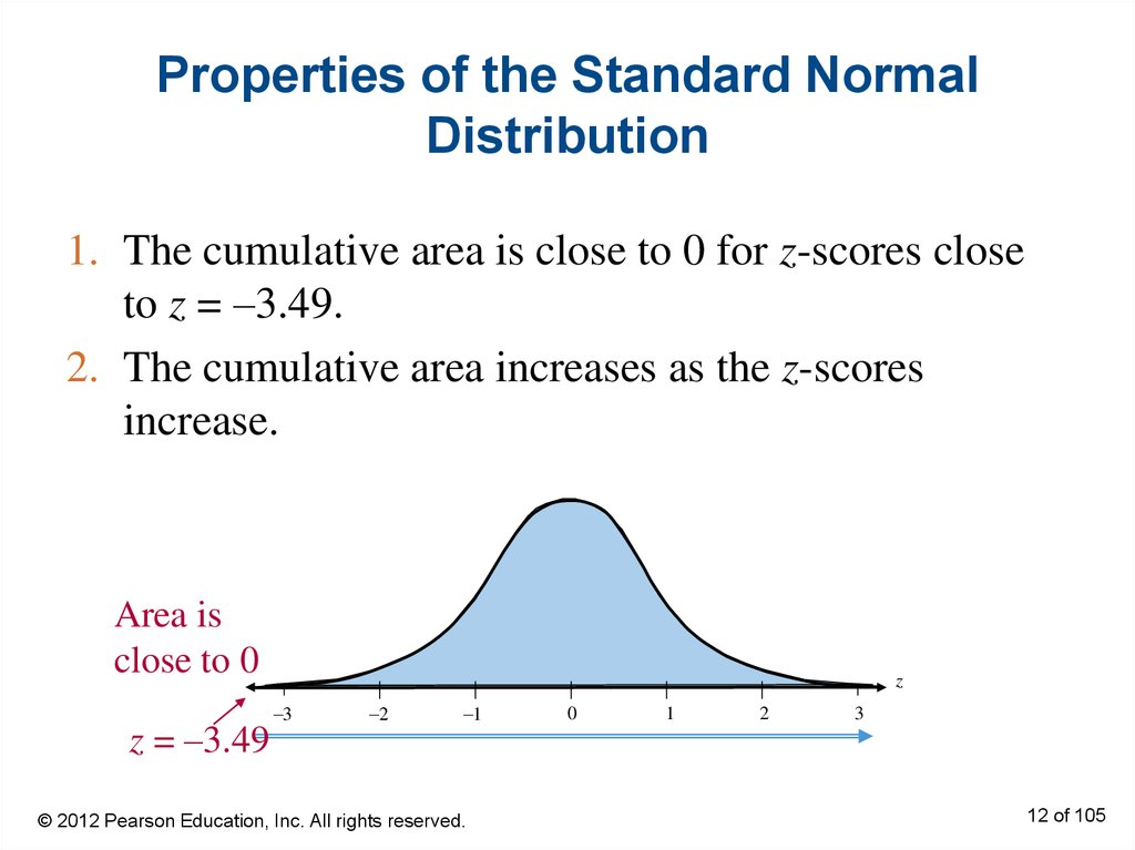
12. Properties of the Standard Normal Distribution
1. The cumulative area is close to 0 for z-scores closeto z = –3.49.
2. The cumulative area increases as the z-scores
increase.
Area is
close to 0
z = –3.49
z
–3
–2
–1
© 2012 Pearson Education, Inc. All rights reserved.
0
1
2
3
12 of 105
13. Properties of the Standard Normal Distribution
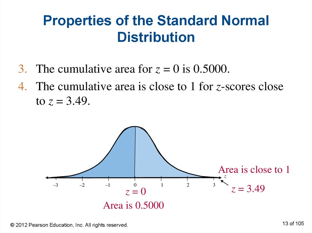
3. The cumulative area for z = 0 is 0.5000.4. The cumulative area is close to 1 for z-scores close
to z = 3.49.
Area
is close to 1
z
–3
–2
–1
0
1
z=0
Area is 0.5000
© 2012 Pearson Education, Inc. All rights reserved.
2
3
z = 3.49
13 of 105
14. Example: Using The Standard Normal Table
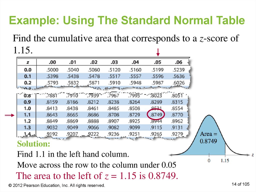
Find the cumulative area that corresponds to a z-score of1.15.
Solution:
Find 1.1 in the left hand column.
Move across the row to the column under 0.05
The area to the left of z = 1.15 is 0.8749.
© 2012 Pearson Education, Inc. All rights reserved.
14 of 105
15. Example: Using The Standard Normal Table
Find the cumulative area that corresponds to a z-score of–0.24.
Solution:
Find –0.2 in the left hand column.
Move across the row to the column under 0.04
The area to the left of z = –0.24 is 0.4052.
© 2012 Pearson Education, Inc. All rights reserved.
15 of 105
16. Finding Areas Under the Standard Normal Curve
1. Sketch the standard normal curve and shade theappropriate area under the curve.
2. Find the area by following the directions for each
case shown.
a. To find the area to the left of z, find the area that
corresponds to z in the Standard Normal Table.
2.
The area to the left
of z = 1.23 is 0.8907
1. Use the table to find the
area for the z-score
© 2012 Pearson Education, Inc. All rights reserved.
16 of 105
17. Finding Areas Under the Standard Normal Curve
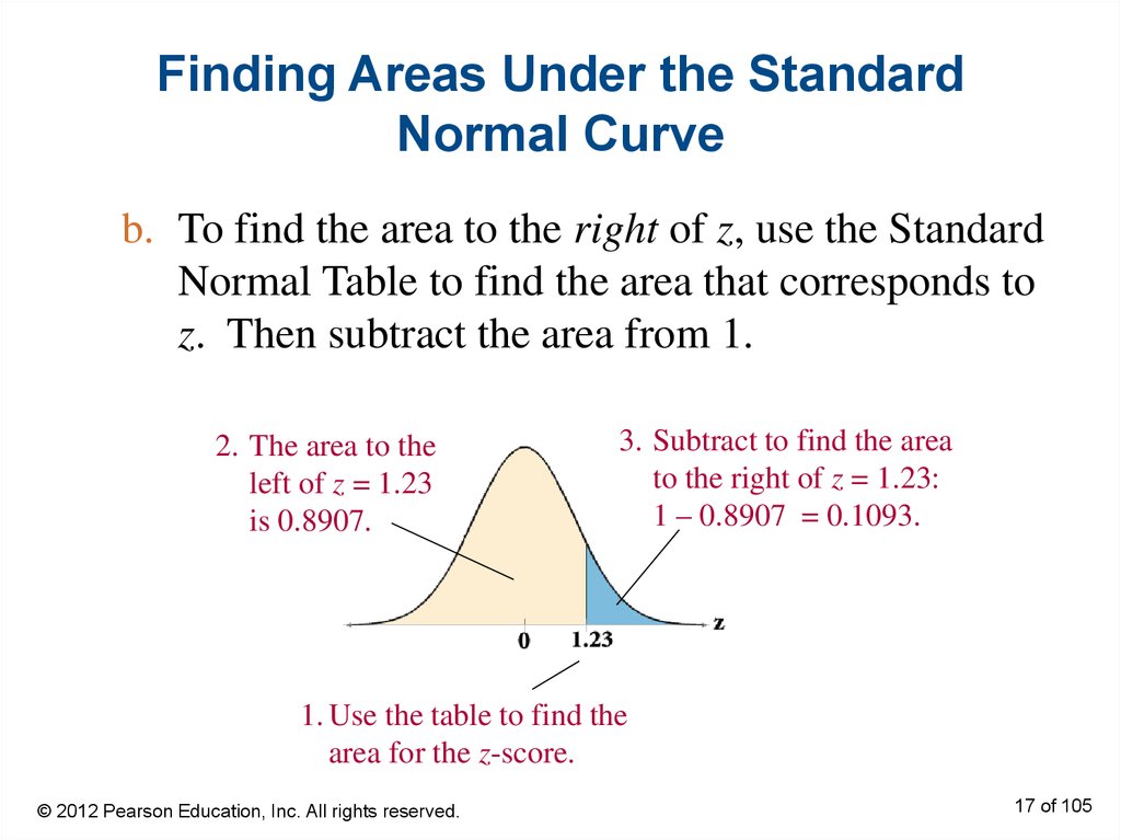
b. To find the area to the right of z, use the StandardNormal Table to find the area that corresponds to
z. Then subtract the area from 1.
2. The area to the
left of z = 1.23
is 0.8907.
3. Subtract to find the area
to the right of z = 1.23:
1 – 0.8907 = 0.1093.
1. Use the table to find the
area for the z-score.
© 2012 Pearson Education, Inc. All rights reserved.
17 of 105
18. Finding Areas Under the Standard Normal Curve
c. To find the area between two z-scores, find thearea corresponding to each z-score in the
Standard Normal Table. Then subtract the
smaller area from the larger area.
2. The area to the
left of z = 1.23
is 0.8907.
3. The area to the
left of z = –0.75
is 0.2266.
4. Subtract to find the area of
the region between the two
z-scores:
0.8907 – 0.2266 = 0.6641.
1. Use the table to find the
area for the z-scores.
© 2012 Pearson Education, Inc. All rights reserved.
18 of 105
19. Example: Finding Area Under the Standard Normal Curve
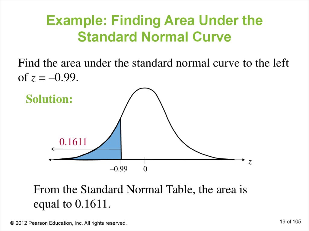
Find the area under the standard normal curve to the leftof z = –0.99.
Solution:
0.1611
–0.99
z
0
From the Standard Normal Table, the area is
equal to 0.1611.
© 2012 Pearson Education, Inc. All rights reserved.
19 of 105
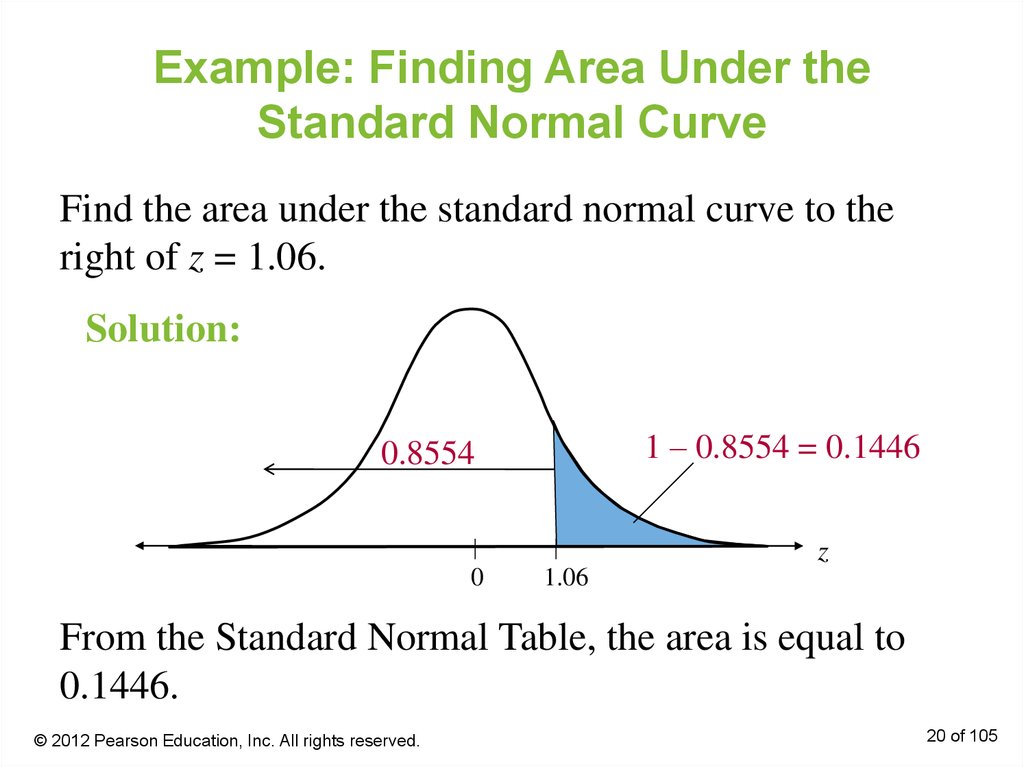
20. Example: Finding Area Under the Standard Normal Curve
Find the area under the standard normal curve to theright of z = 1.06.
Solution:
1 – 0.8554 = 0.1446
0.8554
z
0
1.06
From the Standard Normal Table, the area is equal to
0.1446.
© 2012 Pearson Education, Inc. All rights reserved.
20 of 105
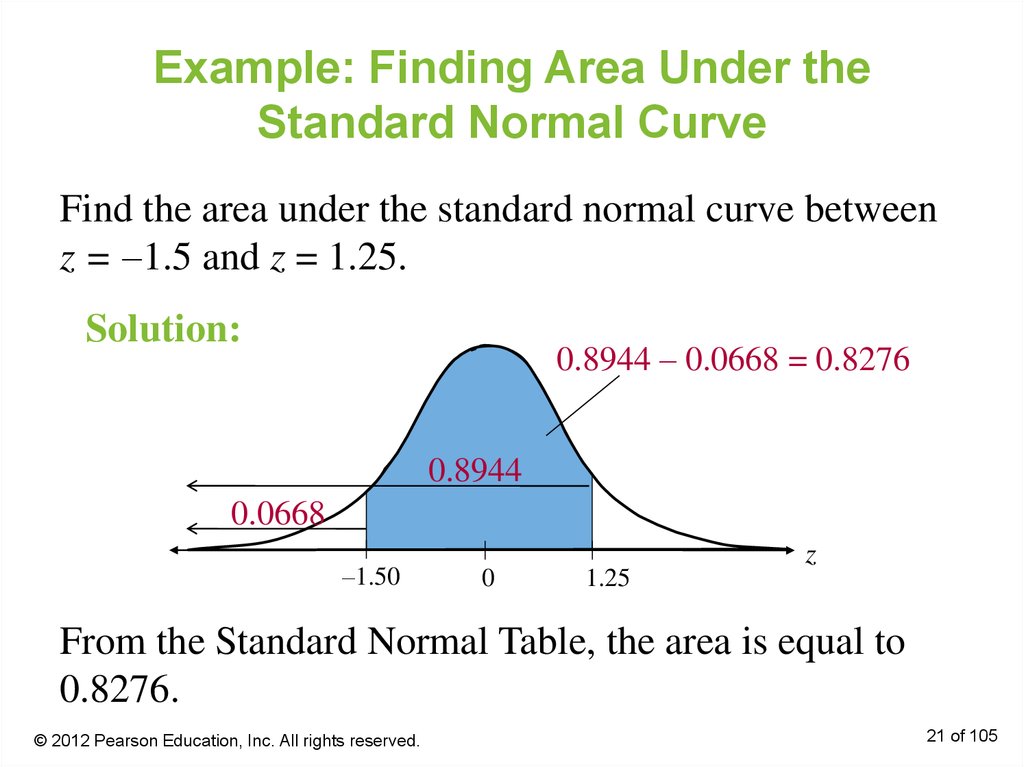
21. Example: Finding Area Under the Standard Normal Curve
Find the area under the standard normal curve betweenz = –1.5 and z = 1.25.
Solution:
0.8944 – 0.0668 = 0.8276
0.8944
0.0668
–1.50
0
1.25
z
From the Standard Normal Table, the area is equal to
0.8276.
© 2012 Pearson Education, Inc. All rights reserved.
21 of 105







 Математика


