Modelling and Simulation IS 331. Lec (5)

1. IS 331

Faculty of Information Technology
Fall 2020
Modelling and Simulation
IS 331
Lec (5)
By Dr. Alaa Zaghloul

2.

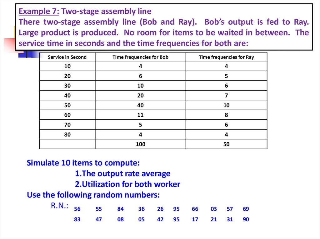
Example 7: Two-stage assembly line
There two-stage assembly line (Bob and Ray). Bob’s output is fed to Ray.
Large product is produced. No room for items to be waited in between. The
service time in seconds and the time frequencies for both are:
Service in Second
Time frequencies for Bob
Time frequencies for Ray
10
4
4
20
6
5
30
10
6
40
20
7
50
40
10
60
11
8
70
5
6
80
4
4
100
50
Simulate 10 items to compute:
1.The output rate average
2.Utilization for both worker
Use the following random numbers:
R.N.: 56
55
84
36
26
95
83
47
08
05
42
95
66
03
57
69
17
21
31
90

3.

Solution 7: Two-stage assembly line
Service (second)
Time frequency
for 1st line Bob
R.N. Allocation
Time frequency
for 2ndline Ray
R.N. Allocation
10
4 0.04
00-03
4 0.08
00-07
20
6 0.06
04-09
5 0.10
08-17
30
10 0.01
10-19
6 0.12
18-29
40
20 0.20
20-39
7 0.14
30-43
50
40 0.40
40-79
10 0.20
44-63
60
11 0.11
80-90
8 0.16
64-79
70
5 0.50
91-95
6 0.12
80-91
80
4 0.04
96-99
4 0.08
92-99
100
50*2=100

4.

Item
No.
56
55
84
36
26
95
66
03
57
69
83
47
08
05
42
95
17
21
31
90
First (Bob) Line
Waiting
Time
R.N
Start
Time
Service
Time
Finish
Time
1
56
00
50
50
2
55
50
50
3
84
120
4
36
5
Second (Ray) Line
R.N
Start
Time
Service
Time
Finish
Time
0
83
50
70
120
100
20
47
120
50
170
60
180
0
08
180
20
200
180
40
220
0
05
220
10
230
26
220
40
260
0
42
260
40
300
6
95
260
70
330
0
95
330
80
410
7
66
330
50
380
30
17
410
20
430
8
03
410
10
420
10
21
430
30
460
9
57
430
50
480
0
31
480
40
520
10
69
480
50
530
0
90
530
70
600
470
60
430

5.

Item
No.
First (Bob) Line
Waiting
Time
R.N
Start
Time
Service
Time
Finish
Time
1
56
00
50
50
2
55
50
50
3
84
120
4
36
5
Second (Ray) Line
R.N
Start
Time
Service
Time
Finish
Time
0
83
50
70
120
100
20
47
120
50
170
60
180
0
08
180
20
200
180
40
220
0
05
220
10
230
26
220
40
260
0
42
260
40
300
6
95
260
70
330
0
95
330
80
410
7
66
330
50
380
30
17
410
20
430
8
03
410
10
420
10
21
430
30
460
9
57
430
50
480
0
31
480
40
520
10
69
480
50
530
0
90
530
70
600
470
60
430
- Output rate average = Total time/No. Of. Product = 600/10=60 sec
- Utilization of Bob line = Total of service time/finish-start time ==470/530-0=88.7%
- Utilization of Ray line = Total of service time/Finish-start time= 430/600-50=78.2%

6.

Example 8: A service station has one gasoline pump. Because everyone
drives big cars, there is room at the station for only three cars including
the car at the pump. Cars arriving where there are already three cars at
the station drive on to another station, Use the following probability
distribution to simulate the arrival of 10 cars to the station.
Inter arrival time (min)
P(X)
Service time (min)
P(X)
10
0.40
5
0.45
20
0.35
10
0.30
30
0.20
15
0.20
40
0.05
33
0.05
Calculate the average time cars spend at the station, the percentage
the station is idle, the utilization of the pump and the average car’s
waiting time.
Use the following R.N:06 95 04 96 26 95 06 99 07 99 03 97 08 95 42 95
42 95 17 99 31 99

7.

Solution 8: gasoline pump
Inter arrival time (min)
P(X)
Service time (min)
P(X)
10
0.40
00—39
5
0.45
00—44
20
0.35
40—74
10
0.30
45—74
30
0.20
75—94
15
0.20
75—94
40
0.05
95—99
33
0.05
95—99

8.

Car#
R.N
interarrival
arrive
No. of
R.N
Service
ON
OFF
cars in
station
Waiting
time
Idle
time
1
06
10
10
1
95
33
10
43
0
10
2
04
10
20
2
96
33
43
76
23
0
3
26
10
30
3
95
33
76
109
46
0
4
06
10
40
5
99
40
80
2
07
5
109
114
29
0
6
99
40
120
1
03
5
120
125
0
6
7
97
40
160
1
08
5
160
165
0
35
8
95
40
200
1
42
5
200
205
0
35
9
95
40
240
1
17
5
240
245
0
35
10
99
40
280
1
31
5
280
285
0
35
98
156
129
The percentage the station is idle =
* 100 = 54.73%
Average time cars spend at the station =Service time+ waiting time/9
=
= 25.22 min
The utilization of the pump =Total of service time/off-start=
* 100 =
45.26%
The average car’s waiting time = = 10.88 min
Idle time = 10 + 6 + 35 +35+35+35= 156 min

9.

Example 9:
Professional football coach has six running backs on his squad. He wants to
evaluate how injuries might affect his stocks of running backs. A minor injury
causes a player to be removed from the game and miss only the next game.
A major injury puts the player out of action for the rest of the season. The
probability of a major in a game is 0.05. There is at most one major injury
per game. The probability of minor injury per game is:
Number of injury
0
1
2
3
4
5
Probability
0.2
0.5
0.22
0.05
0.025
0.005
Injuries seem to happen in a completely random pattern over the season. A
season is 10 games. Using the following random number, simulate the
fluctuating in the coach’s stock of running backs over the season. Assume that
he hires no additional running backs during the season:R.N:
044 392 898 615 986 959 558 353 577 866 305 813 024 189 878 023
285 442 862 848 060 131 963 874 805 105 452

10.

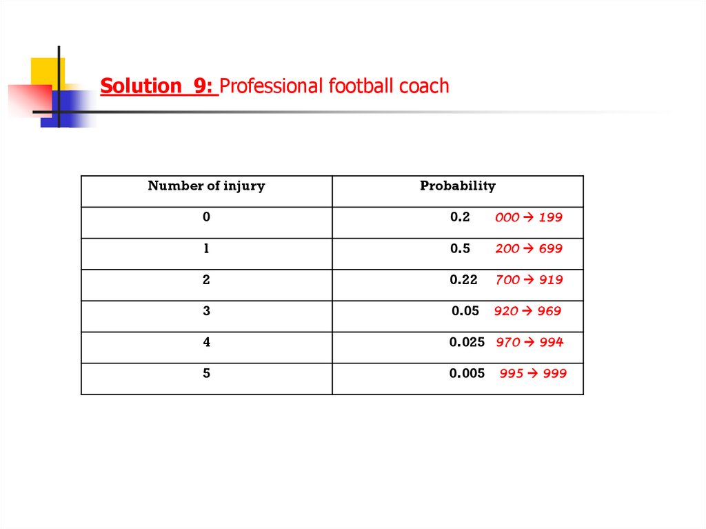
Solution 9: Professional football coach
Number of injury
Probability
0
0.2
000 199
1
0.5
200 699
2
0.22
700 919
3
0.05 920 969
4
0.025 970 994
5
0.005 995 999

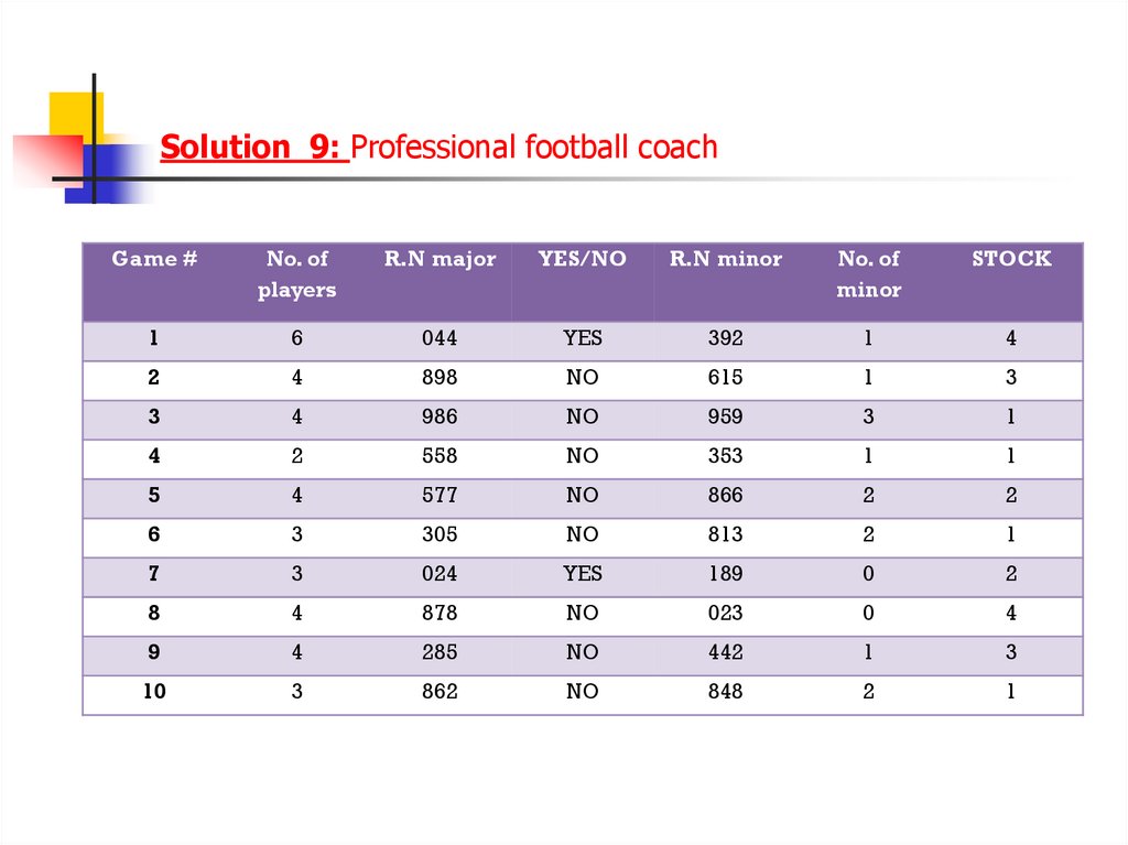
11.

Solution 9: Professional football coach
Game #
No. of
players
R.N major
YES/NO
R.N minor
No. of
minor
STOCK
1
6
044
YES
392
1
4
2
4
898
NO
615
1
3
3
4
986
NO
959
3
1
4
2
558
NO
353
1
1
5
4
577
NO
866
2
2
6
3
305
NO
813
2
1
7
3
024
YES
189
0
2
8
4
878
NO
023
0
4
9
4
285
NO
442
1
3
10
3
862
NO
848
2
1

12.

END