 Физика
Похожие презентации:


New regular solutions with axial symmetry in Einstein–Yang–Mills theory
1.
Physics Letters B 609 (2005) 150–156www.elsevier.com/locate/physletb
New regular solutions with axial symmetry
in Einstein–Yang–Mills theory
Rustam Ibadov a , Burkhard Kleihaus b , Jutta Kunz b , Yasha Shnir b
a Department of Theoretical Physics and Computer Science, Samarkand State University, Samarkand, Usbekistan
b Institut für Physik, Universität Oldenburg, Postfach 2503, D-26111 Oldenburg, Germany
Received 20 October 2004; accepted 16 January 2005
Available online 25 January 2005
Editor: L. Alvarez-Gaumé
Abstract
We construct new regular solutions in Einstein–Yang–Mills theory. They are static, axially symmetric and asymptotically flat.
They are characterized by a pair of integers (k, n), where k is related to the polar angle and n to the azimuthal angle. The known
spherically and axially symmetric EYM solutions have k = 1. For k > 1 new solutions arise, which form two branches. They
exist above a minimal value of n, that increases with k. The solutions on the lower mass branch are related to certain solutions
of Einstein–Yang–Mills–Higgs theory, where the nodes of the Higgs field form rings.
2005 Elsevier B.V. All rights reserved.
1. Introduction
The well-known regular Bartnik–McKinnon (BM)
solutions [1] and the corresponding non-Abelian black
hole solutions [2], are asymptotically flat, static spherically symmetric solutions of SU(2) Einstein–Yang–
Mills (EYM) theory. They are unstable solutions,
sphalerons [3], and are characterized by the number
of nodes of the gauge field. Besides the BM solutions
there are also asymptotically flat, static, only axially
symmetric regular and black hole solutions [4]. These
E-mail address: kleihaus@marvin.physik.uni-oldenburg.de
(B. Kleihaus).
0370-2693/$ – see front matter 2005 Elsevier B.V. All rights reserved.
doi:10.1016/j.physletb.2005.01.038
are characterized by two integers, the node number of
their gauge field function(s), and the winding number
with respect to the azimuthal angle, denoted n. The
spherically symmetric solutions have winding number n = 1, while the axially symmetric solutions have
winding number n > 1.
In SU(2) Einstein–Yang–Mills–Higgs (EYMH)
theory, with a triplet Higgs field, gravitating monopole
solutions arise [5]. While gravitating monopoles with
unit magnetic charge are spherically symmetric, the
known gravitating multimonopoles possess axial symmetry [6]. As in EYM theory, these EYMH solutions
are characterized by two integers, the node number
of the gauge field and the azimuthal winding num-
2.
R. Ibadov et al. / Physics Letters B 609 (2005) 150–156ber n, which corresponds to the topological charge of
the monopoles.
But EYMH theory allows for further static axially symmetric solutions, representing gravitating
monopole–antimonopole pair, chain and vortex solutions [7–9]. These solutions can be characterized
by the azimuthal winding number n, and by a second integer m, related to the polar angle. For the
monopole–antimonopole chains, which in flat space
arise for n = 1 and 2, the integer m corresponds to
the number of nodes of the Higgs field (and thus the
number of poles on the symmetry axis) [8]. In vortex solutions, on the other hand, which in flat space
arise for winding number n > 2, the Higgs field vanishes (for even m) on m/2 rings centered around the
symmetry axis [8].
The existence of monopole–antimonopole pair,
chain and vortex solutions in EYMH theory [7–9] immediately leads to the question, whether there might
be analogous solutions in EYM theory, even though
there would be no Higgs field participating in the
subtle interplay of attraction and repulsion. In this
Letter we report the existence of one such new type
of solution, related to vortex solutions in EYMH theory.
In Section 2 we present the EYM action, the axially symmetric ansatz and the boundary conditions. In
Section 3 we discuss the properties of the new axially
symmetric solutions, and we present our conclusions
in Section 4.
2. Action and ansatz
We consider the SU(2) EYM action
S=
√
1
R
− Tr Fµν F µν
−g d 4 x
16πG 2
(1)
with Ricci scalar R, field strength tensor
Fµν = ∂µ Aν − ∂ν Aµ + ie[Aµ , Aν ],
(2)
gauge potential Aµ =
and gravitational and
Yang–Mills coupling constants G and e, respectively.
Variation of the action (1) with respect to the metτ a Aaµ /2,
151
ric g µν leads to the Einstein equations, variation with
respect to the gauge potential Aµ to the gauge field
equations.
In isotropic coordinates the static axially symmetric
metric reads [4]
ds 2 = −f dt 2 +
+
m 2 mr 2 2
dr +
dθ
f
f
lr 2 sin2 θ
dϕ 2 ,
f
(3)
where the metric functions f , m and l are functions of
the coordinates r and θ , only. The z-axis (θ = 0, π )
represents the symmetry axis. Regularity on the z-axis
requires m = l there.
For the gauge field we employ the ansatz [4,8,9]
Aµ dx µ =
1 n
τ H1 dr + (1 − H2 )r dθ
2er ϕ
− n τrn,k H3 + τθn,k H4 r sin θ dφ .
(4)
Here the symbols τrn,k , τθn,k and τϕn denote the dot
products of the Cartesian vector of Pauli matrices,
τ = (τx , τy , τz ), with the spatial unit vectors
e rn,k = (sin kθ cos nϕ, sin kθ sin nϕ, cos kθ ),
e θn,k = (cos kθ cos nϕ, cos kθ sin nϕ, − sin kθ ),
e ϕn = (− sin nϕ, cos nϕ, 0),
(5)
respectively. The gauge field functions Hi , i =
1, . . . , 4, depend on the coordinates r and θ , only. For
k = n = 1 and H1 = H3 = 0, H2 = 1 − H4 = w(r)
the BM solutions [1] are recovered, while for k = 1,
n > 1, one obtains the axially symmetric solutions
of [4]. The new solutions reported here are obtained
for k > 1. They are related to EYMH solutions with
m = 2k in the limit of vanishing Higgs field [9].
The ansatz is form-invariant under the Abelian
gauge transformation [4]
i n
U = exp τφ Γ (r, θ ) .
2
(6)
We fix the gauge by choosing the gauge condition
[4,8,9]
r∂r H1 − ∂θ H2 = 0.
(7)
3.
152R. Ibadov et al. / Physics Letters B 609 (2005) 150–156
To obtain asymptotically flat solutions which are
globally regular and possess the proper symmetries,
we need to impose appropriate boundary conditions
[4,8,9]. At the origin we impose the boundary conditions
∂r f = ∂r m = ∂r l = 0,
H1 = H3 = H4 = 0,
H2 = 1,
(8)
at infinity we impose
f = m = l = 1,
H1 = H3 = 0,
H2 = 1 − 2k,
H4 = 2 sin(kθ )/ sin θ,
(9)
and on the z-axis we impose
∂θ f = ∂θ m = ∂θ l = 0,
H1 = H3 = 0,
∂θ H2 = ∂θ H4 = 0.
(10)
We further introduce the dimensionless coordinate x, and the dimensionless mass µ,
e
x=√
r,
4πG
eG
µ= √
M.
4πG
(11)
3. Numerical results
Subject to the above boundary conditions, we solve
the system of seven coupled nonlinear partial differential equations numerically. To map spatial infinity to
the finite value x̄ = 1, we employ the radial coordinate
[4,8,9]
x̄ =
x
.
1+x
(12)
The numerical calculations are based on the Newton–
Raphson method, and are performed with help of the
program FIDISOL [10]. The equations are discretized
on a nonequidistant grid in x̄ and θ . Typical grids
used have sizes 70 × 30, covering the integration region 0 x̄ 1 and 0 θ π/2. For the method, it is
essential to have a good first guess, to start the iteration
procedure. For the k = 1 EYM solutions, the n = 1
BM solutions serve as a first guess, and then the ‘parameter’ n is varied (via unphysical noninteger values)
to obtain solutions with higher winding number n [4].
For the k = 2 solutions we employ the m = 4, n = 4
EYMH vortex solution with (almost) vanishing Higgs
field as a first guess [9], and then again vary n. Similarly, for the k = 3 solutions we start from the m = 6,
n = 6 EYMH vortex solution.
In EYMH theory, the monopole–antimonopole pair
(MAP) solution is obtained, when m = 2k = 2, n = 1.
Here a monopole and an antimonopole are located
symmetrically on the z-axis. Similarly, one might try
to find a sphaleron–antisphaleron pair (SAP) solution
in EYM theory. The boundary conditions of such a
SAP solution, however, do not differ from those of
a BM solution. Consequently,
when the EYMH cou√
pling constant α = 4πGv (where v is the Higgs
field expectation value) is varied, the gravitating MAP
solution starts from the flat space solution, reaches a
critical solution at a maximal value of α, and then
with decreasing α smoothly reaches the BM solution
in the limit α → 0 (after rescaling of the radial coordinate) [7]. Consequently, we do not find a SAP solution
in EYM theory, and similarly, we do not find new solutions, when m = 2k = 2, n > 1, since their boundary
conditions agree with those of the axially symmetric
solutions of [4].
When m = 2k = 4, however, the boundary conditions Eq. (9) for the gauge field differ from those of
the known solutions [1,4]. We therefore may expect
the existence of new EYM solutions, subject to these
boundary conditions. Indeed, for m = 4, n = 4, for instance, when α is varied again, the gravitating EYMH
vortex solution starts from the flat space solution [8],
reaches a critical solution at a maximal value of α, and
then with decreasing α smoothly reaches a new EYM
solution in the limit α → 0 (after rescaling of the radial coordinate) [9].
Let us in the following refer to the solutions characterized by the integers k and n as (k, n) solutions.
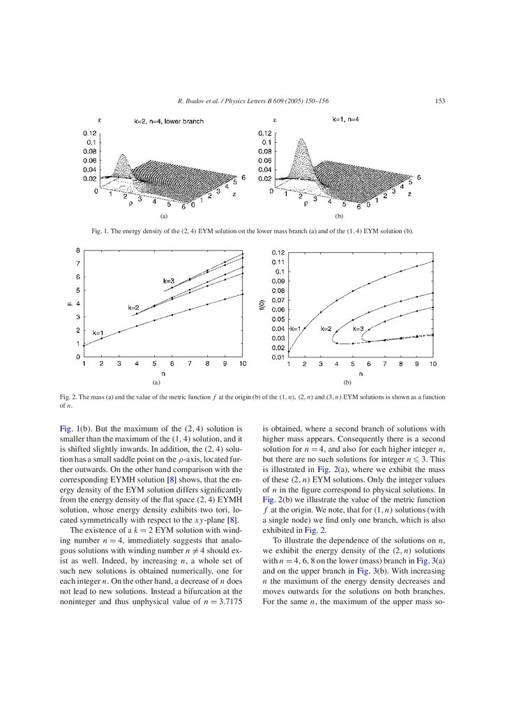
In Fig. 1(a) we exhibit the energy density of the new
(2, 4) EYM solution. Its energy density has a pronounced maximum on the ρ-axis, thus the energy density is torus-like. The energy density of this (2, 4) solution is thus similar to the energy density of the (lowest
mass) known (1, 4) EYM solution [4], exhibited in
4.
R. Ibadov et al. / Physics Letters B 609 (2005) 150–156(a)
153
(b)
Fig. 1. The energy density of the (2, 4) EYM solution on the lower mass branch (a) and of the (1, 4) EYM solution (b).
(a)
(b)
Fig. 2. The mass (a) and the value of the metric function f at the origin (b) of the (1, n), (2, n) and (3, n) EYM solutions is shown as a function
of n.
Fig. 1(b). But the maximum of the (2, 4) solution is
smaller than the maximum of the (1, 4) solution, and it
is shifted slightly inwards. In addition, the (2, 4) solution has a small saddle point on the ρ-axis, located further outwards. On the other hand comparison with the
corresponding EYMH solution [8] shows, that the energy density of the EYM solution differs significantly
from the energy density of the flat space (2, 4) EYMH
solution, whose energy density exhibits two tori, located symmetrically with respect to the xy-plane [8].
The existence of a k = 2 EYM solution with winding number n = 4, immediately suggests that analogous solutions with winding number n = 4 should exist as well. Indeed, by increasing n, a whole set of
such new solutions is obtained numerically, one for
each integer n. On the other hand, a decrease of n does
not lead to new solutions. Instead a bifurcation at the
noninteger and thus unphysical value of n = 3.7175
is obtained, where a second branch of solutions with
higher mass appears. Consequently there is a second
solution for n = 4, and also for each higher integer n,
but there are no such solutions for integer n 3. This
is illustrated in Fig. 2(a), where we exhibit the mass
of these (2, n) EYM solutions. Only the integer values
of n in the figure correspond to physical solutions. In
Fig. 2(b) we illustrate the value of the metric function
f at the origin. We note, that for (1, n) solutions (with
a single node) we find only one branch, which is also
exhibited in Fig. 2.
To illustrate the dependence of the solutions on n,
we exhibit the energy density of the (2, n) solutions
with n = 4, 6, 8 on the lower (mass) branch in Fig. 3(a)
and on the upper branch in Fig. 3(b). With increasing
n the maximum of the energy density decreases and
moves outwards for the solutions on both branches.
For the same n, the maximum of the upper mass so-
5.
154R. Ibadov et al. / Physics Letters B 609 (2005) 150–156
(a)
(b)
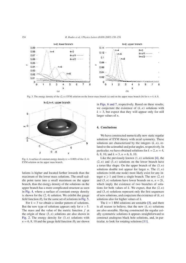
Fig. 3. The energy density of the (2, n) EYM solution on the lower mass branch (a) and on the upper mass branch (b) for n = 4, 6, 8.
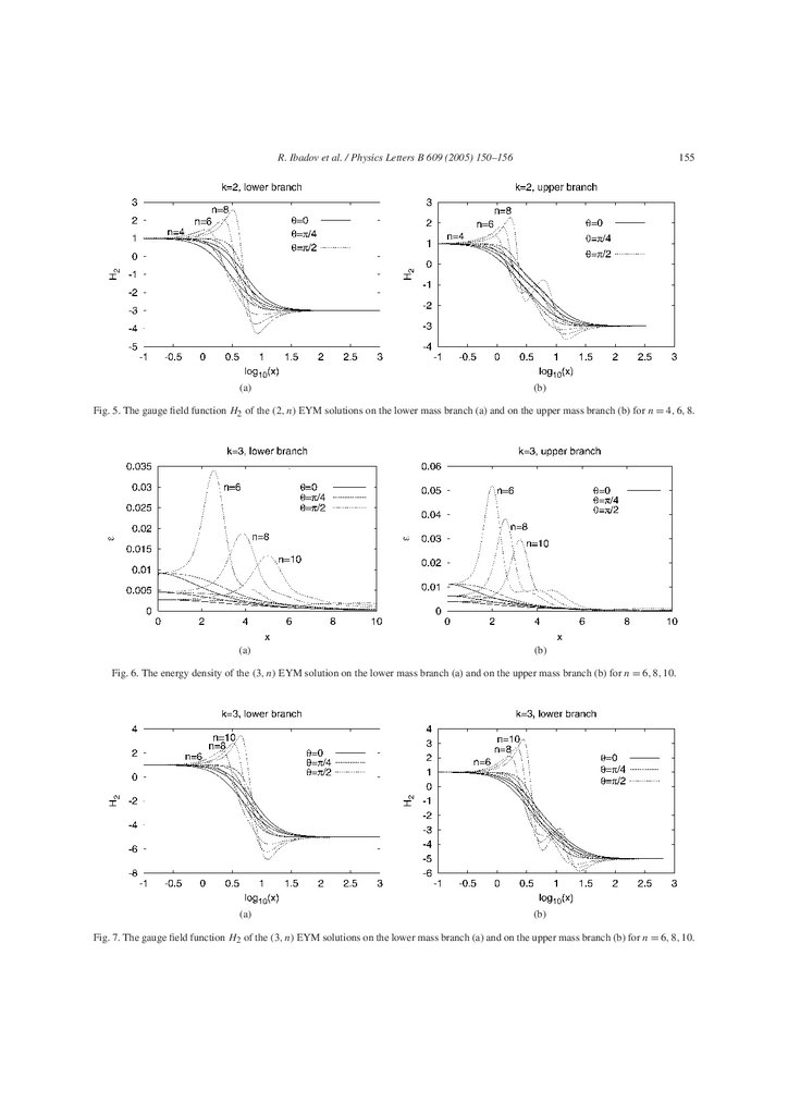
in Figs. 6 and 7, respectively. Based on these results,
we conjecture the existence of (k, n) solutions with
k > 3, but expect that they will appear only for still
larger values of n.
4. Conclusions
Fig. 4. A surface of constant energy density (ε = 0.005) of the (2, 4)
EYM solution on the upper mass branch.
lutions is higher and located further inwards than the
maximum of the lower mass solutions. The small saddle point turns into a small maximum on the upper
branch, thus the energy density of the solutions on the
upper branch has a more complicated structure as seen
in Fig. 4, where a surface of constant energy density
is shown for the (2, 4) solution. We exhibit the gauge
field function H2 for the same set of solutions in Fig. 5.
For k = 3 we obtain a similar pattern of solutions.
But the new type of solutions appears only for n > 5.
The mass and the value of the metric function f at
the origin of these (3, n) solutions are also shown in
Fig. 2. The energy density for (3, n) solutions with
n = 6, 8, 10 and the gauge field function H2 are shown
We have constructed numerically new static regular
solutions of EYM theory with axial symmetry. These
solutions are characterized by the integers (k, n), related to the azimuthal and polar angles, respectively. In
particular, we have obtained solutions for k = 2, n = 4,
6, 8, 10, and k = 3, n = 6, 8, 10.
Like the previously known (1, n) solutions [4], the
(2, n) and (3, n) solutions on the lower branch have
a torus-like shape. On the upper branch of the (3, n)
solutions double tori appear for larger n. The (1, n)
solutions (with one node) most likely exist for any integer n 1 and form a single branch. The new (2, n)
and (3, n) solutions have lower bounds on n, n = 2k,
which imply the existence of two branches of solutions for both values of k. We expect, that the (2, n)
and (3, n) solutions represent only the first sequences
of new solutions, and conjecture the existence of (k, n)
solutions also for higher values of k.
The k = 1 BM solutions are unstable [3], and there
is all reason to believe, that the new (k, n) solutions
are also unstable. Having constructed the regular axially symmetric solutions it appears straightforward to
construct analogous black hole solutions, and, in particular, to look for rotating solutions [11].
6.
R. Ibadov et al. / Physics Letters B 609 (2005) 150–156(a)
155
(b)
Fig. 5. The gauge field function H2 of the (2, n) EYM solutions on the lower mass branch (a) and on the upper mass branch (b) for n = 4, 6, 8.
(a)
(b)
Fig. 6. The energy density of the (3, n) EYM solution on the lower mass branch (a) and on the upper mass branch (b) for n = 6, 8, 10.
(a)
(b)
Fig. 7. The gauge field function H2 of the (3, n) EYM solutions on the lower mass branch (a) and on the upper mass branch (b) for n = 6, 8, 10.
7.
156R. Ibadov et al. / Physics Letters B 609 (2005) 150–156
Acknowledgements
R.I. gratefully acknowledges support by the DAAD,
and B.K. support by the DFG.
References
[1] R. Bartnik, J. McKinnon, Phys. Rev. Lett. 61 (1988) 141.
[2] M.S. Volkov, D.V. Gal’tsov, Sov. J. Nucl. Phys. 51 (1990) 747;
P. Bizon, Phys. Rev. Lett. 64 (1990) 2844;
H.P. Künzle, A.K.M. Masoud-ul-Alam, J. Math. Phys. 31
(1990) 928.
[3] N. Straumann, Z.H. Zhou, Phys. Lett. B 237 (1990) 353;
N. Straumann, Z.H. Zhou, Phys. Lett. B 243 (1990) 33;
M.S. Volkov, D.V. Gal’tsov, Phys. Lett. B 341 (1995) 279;
G. Lavrelashvili, D. Maison, Phys. Lett. B 343 (1995) 214;
M.S. Volkov, O. Brodbeck, G. Lavrelashvili, N. Straumann,
Phys. Lett. B 349 (1995) 438.
[4] B. Kleihaus, J. Kunz, Phys. Rev. Lett. 78 (1997) 2527;
B. Kleihaus, J. Kunz, Phys. Rev. Lett. 79 (1997) 1595;
B. Kleihaus, J. Kunz, Phys. Rev. D 57 (1998) 834;
B. Kleihaus, J. Kunz, Phys. Rev. D 57 (1998) 6138.
[5] K. Lee, V.P. Nair, E.J. Weinberg, Phys. Rev. D 45 (1992) 2751;
P. Breitenlohner, P. Forgacs, D. Maison, Nucl. Phys. B 383
(1992) 357;
[6]
[7]
[8]
[9]
[10]
[11]
P. Breitenlohner, P. Forgacs, D. Maison, Nucl. Phys. B 442
(1995) 126.
B. Hartmann, B. Kleihaus, J. Kunz, Phys. Rev. Lett. 86 (2001)
1422;
B. Hartmann, B. Kleihaus, J. Kunz, Phys. Rev. D 65 (2002)
024027.
B. Kleihaus, J. Kunz, Phys. Rev. Lett. 85 (2000) 2430.
B. Kleihaus, J. Kunz, Ya. Shnir, Phys. Lett. B 570 (2003) 237;
B. Kleihaus, J. Kunz, Ya. Shnir, Phys. Rev. D 68 (2003)
101701;
B. Kleihaus, J. Kunz, Ya. Shnir, Phys. Rev. D 70 (2004)
065010.
B. Kleihaus, J. Kunz, Ya. Shnir, Phys. Rev. D 71 (2005)
024013.
W. Schönauer, R. Weiß, J. Comput. Appl. Math. 27 (1989) 279;
M. Schauder, R. Weiß, W. Schönauer, The CADSOL Program
Package, Universität Karlsruhe, Interner Bericht Nr. 46/92
(1992).
B. Kleihaus, J. Kunz, Phys. Rev. Lett. 86 (2001) 3704;
B. Kleihaus, J. Kunz, F. Navarro-Lérida, Phys. Rev. D 66
(2002) 104001;
B. Kleihaus, J. Kunz, F. Navarro-Lérida, Phys. Rev. Lett. 90
(2003) 171101;
B. Kleihaus, J. Kunz, F. Navarro-Lérida, Phys. Rev. D 69
(2004) 064028;
B. Kleihaus, J. Kunz, F. Navarro-Lérida, Phys. Lett. B 599
(2004) 294.