Похожие презентации:
Analyzing a Case Study – CS #1. Acoustic
1.
Analyzing A Case StudyCase Study #1
February 2012
2. Analyzing a Case Study – CS #1
Here are the steps when coming to analyze a session:Quick sanity check
Generate a visual reference
Verify parameters. Adjust tube length
Run auto-analysis
Verify auto analysis results
Quick full manual verification
3. Quick sanity check
In order to get general impression of what we are going to deal with, load the session, then go to report>signals, right click on the measurement list and choose “select all measurements”.You can review:
Tubes cleanliness level.
Measurements quality level – noisy or quiet.
Inspection noise conditions.
Write down noisy signals, outliers or signals you don’t want to analyze.
Write down significant defects. Later on we will verify that they were captured by the analysis.
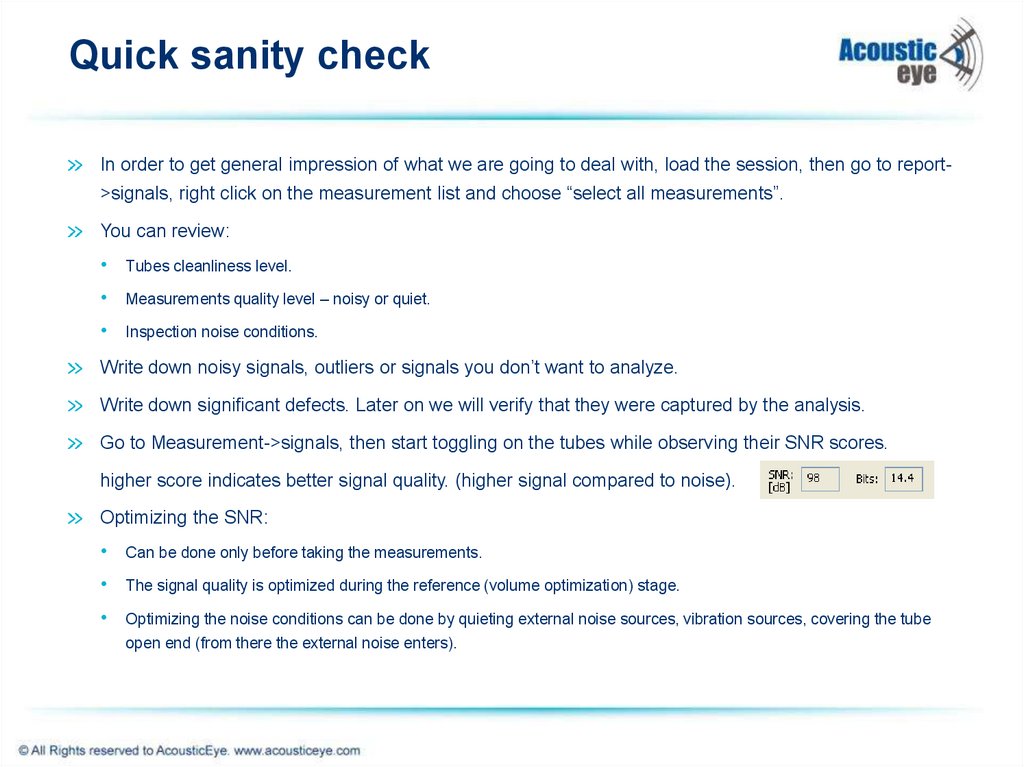
Go to Measurement->signals, then start toggling on the tubes while observing their SNR scores.
higher score indicates better signal quality. (higher signal compared to noise).
Optimizing the SNR:
Can be done only before taking the measurements.
The signal quality is optimized during the reference (volume optimization) stage.
Optimizing the noise conditions can be done by quieting external noise sources, vibration sources, covering the tube
open end (from there the external noise enters).
4. Generate a visual reference
The APR is a comparative method. Faults are detected by comparing a measured tube to a referenceone. The reference measurement represents a faultless tube.
The system is using 2 types of reference tube during the analysis:
• Automatic reference
• Visual reference.
The automatic reference is calculated statistically while running the auto analysis. The user has no
influence on this process. The system is splitting the session into sub-groups of similar behaving signals.
In each group a reference is created by averaging the group tubes, while neglecting outliers.
The visual reference is created by the user. It’s used during the auto analysis results verification phase
(that is the reference taken when applying the “subtract reference” option).
The user can impose the use of the visual reference for the auto analysis using the “impose reference
tube” parameter at the report->option tab. This option is valid When coming to analyze small sized
sessions (<20 tubes), where a reference that is created statistically isn’t strong enough.
5. Generate a visual reference
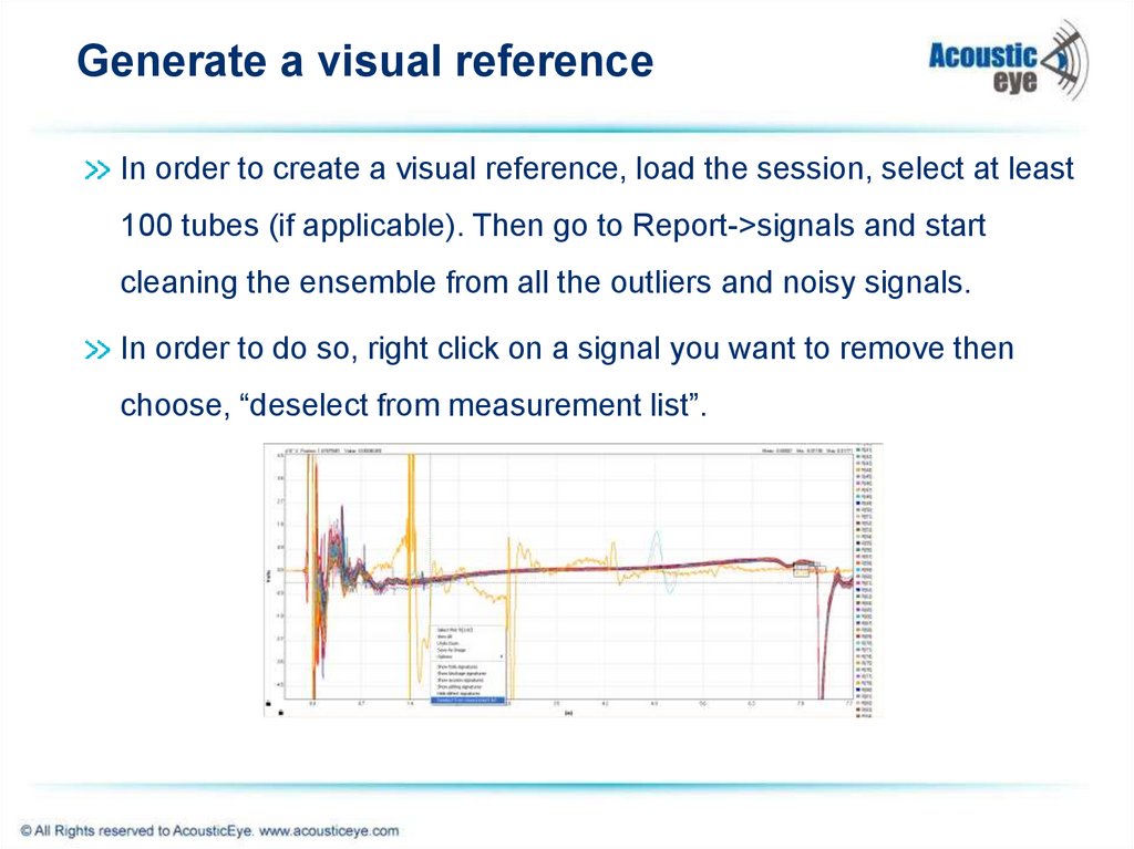
In order to create a visual reference, load the session, select at least100 tubes (if applicable). Then go to Report->signals and start
cleaning the ensemble from all the outliers and noisy signals.
In order to do so, right click on a signal you want to remove then
choose, “deselect from measurement list”.
6. Generate a visual reference
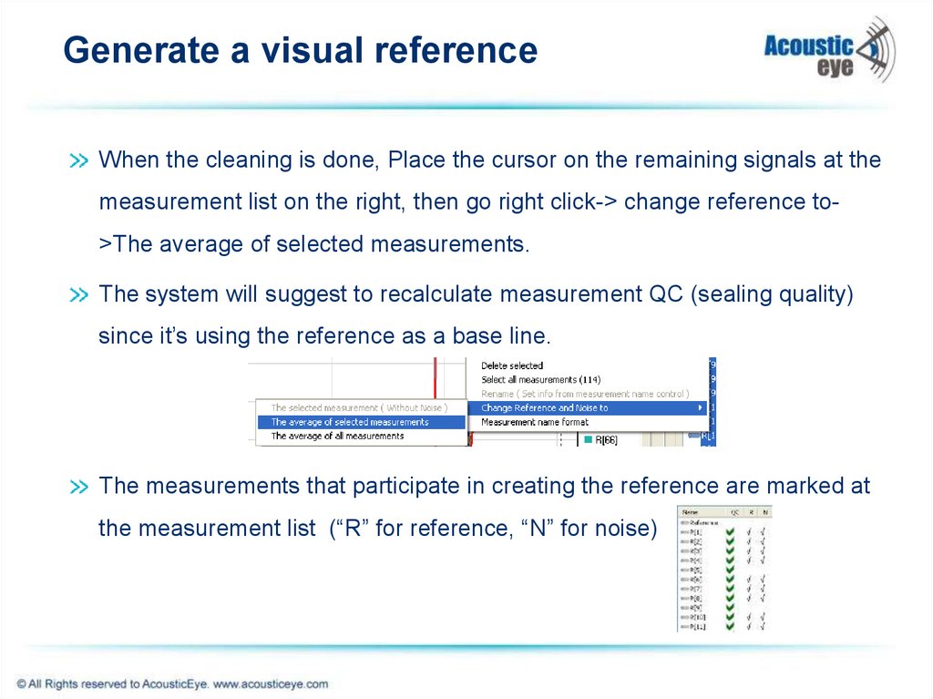
When the cleaning is done, Place the cursor on the remaining signals at themeasurement list on the right, then go right click-> change reference to>The average of selected measurements.
The system will suggest to recalculate measurement QC (sealing quality)
since it’s using the reference as a base line.
The measurements that participate in creating the reference are marked at
the measurement list (“R” for reference, “N” for noise)
7. verify parameters
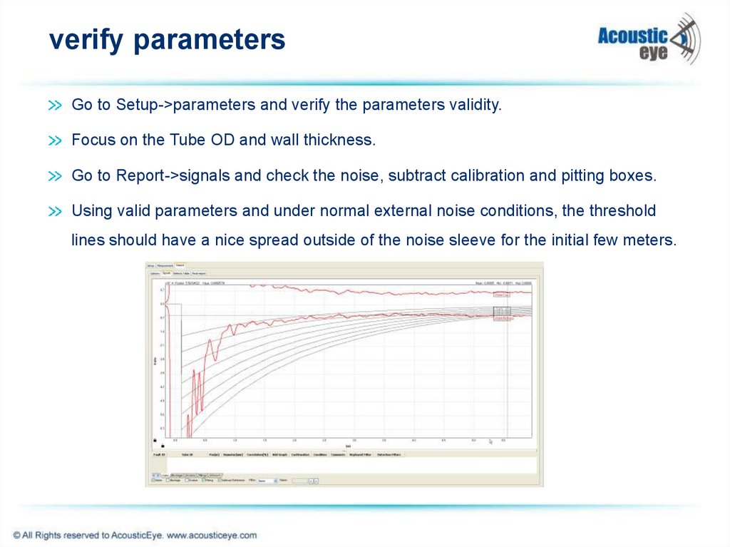
Go to Setup->parameters and verify the parameters validity.Focus on the Tube OD and wall thickness.
Go to Report->signals and check the noise, subtract calibration and pitting boxes.
Using valid parameters and under normal external noise conditions, the threshold
lines should have a nice spread outside of the noise sleeve for the initial few meters.
8. Adjust Tube Length
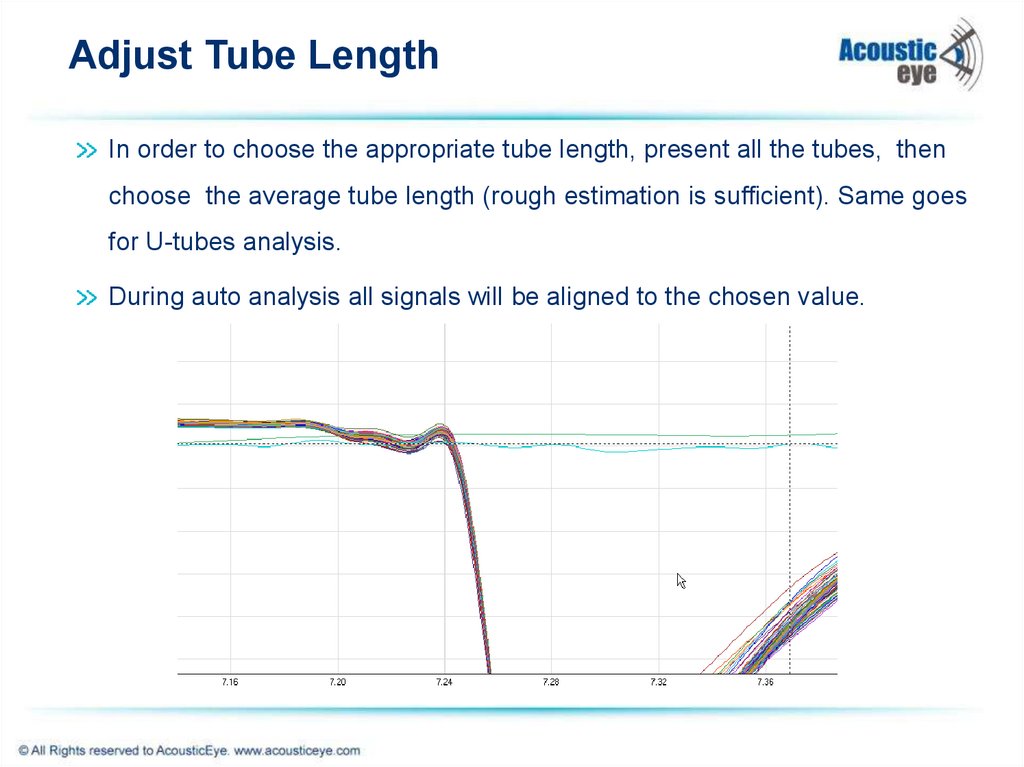
In order to choose the appropriate tube length, present all the tubes, thenchoose the average tube length (rough estimation is sufficient). Same goes
for U-tubes analysis.
During auto analysis all signals will be aligned to the chosen value.
9. Run the Auto-Analysis
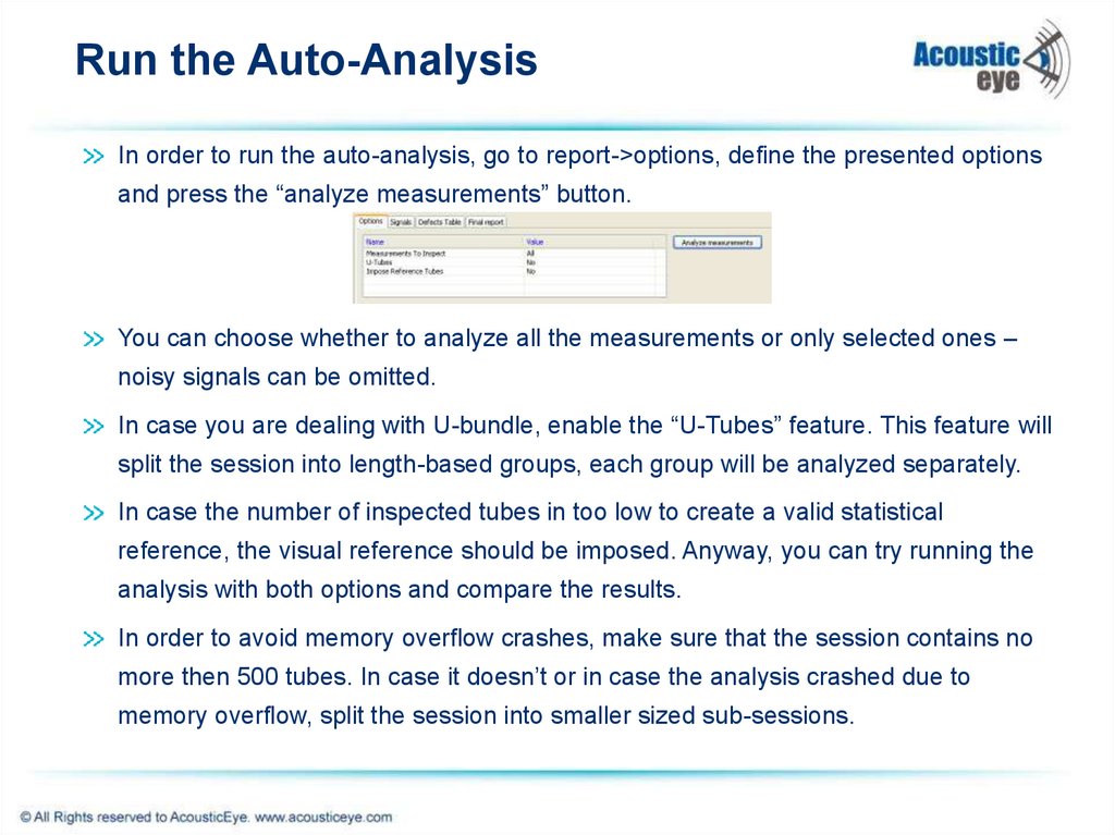
In order to run the auto-analysis, go to report->options, define the presented optionsand press the “analyze measurements” button.
You can choose whether to analyze all the measurements or only selected ones –
noisy signals can be omitted.
In case you are dealing with U-bundle, enable the “U-Tubes” feature. This feature will
split the session into length-based groups, each group will be analyzed separately.
In case the number of inspected tubes in too low to create a valid statistical
reference, the visual reference should be imposed. Anyway, you can try running the
analysis with both options and compare the results.
In order to avoid memory overflow crashes, make sure that the session contains no
more then 500 tubes. In case it doesn’t or in case the analysis crashed due to
memory overflow, split the session into smaller sized sub-sessions.
10. Verifying the auto analysis results
Now starts the second stage of the results analysis – the uservalidation part in which the user verify the system indications.
Pay attention that the algorithms were tuned to be over-sensitive,
therefore you should expect to have false alarms.
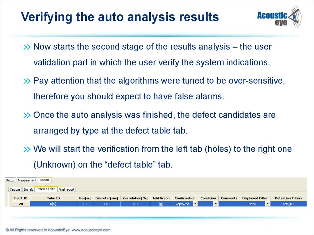
Once the auto analysis was finished, the defect candidates are
arranged by type at the defect table tab.
We will start the verification from the left tab (holes) to the right one
(Unknown) on the “defect table” tab.
11. Verifying the auto analysis results
Just by looking at the initial indications list we can learn someimportant staff that will ease our analysis:
Does a lot of the indications occur at the same place?
Probably false alarms.
Maybe the reference tube is problematic at this location – a
signature caused by a structural change in the tube.
Do I have one tube with a lot of indications? Maybe the signal isn’t
valid (sealing, noise, etc.)
It’s recommended to review the defects after sorting the defect table
by location.
12. Verifying the auto analysis results - Holes
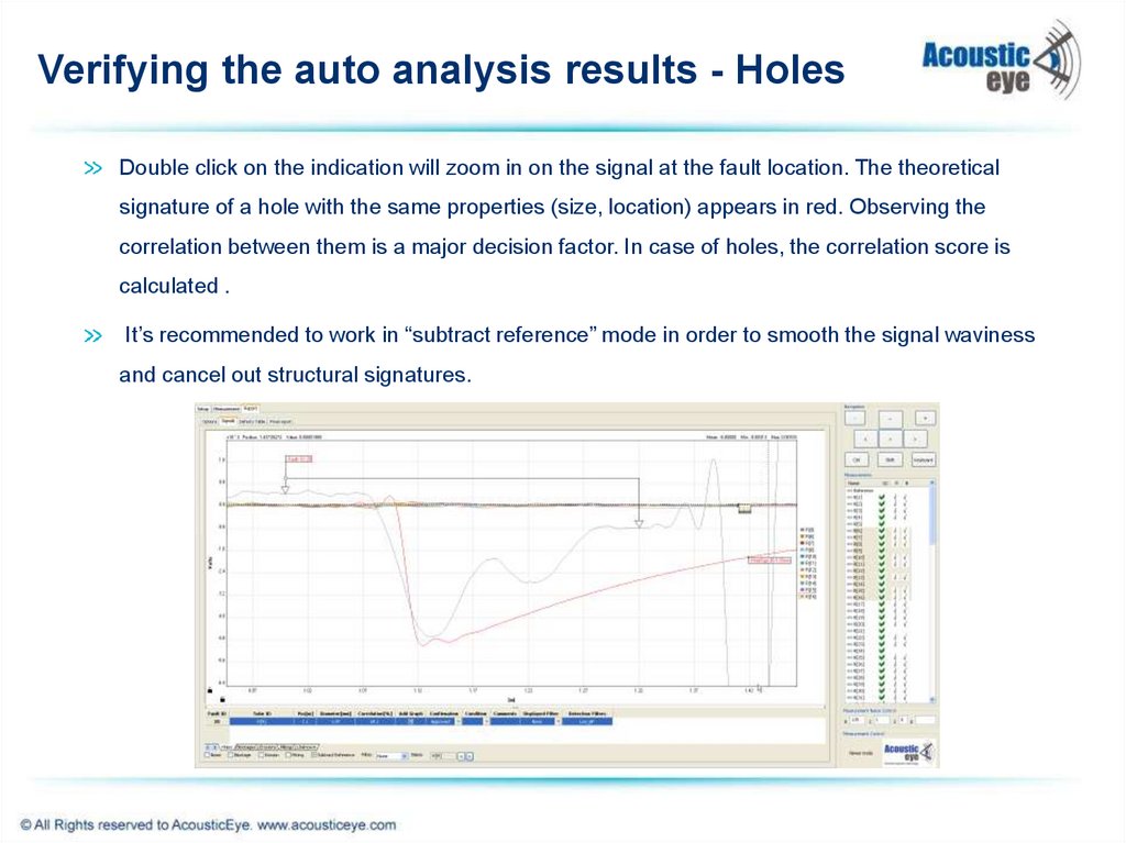
Double click on the indication will zoom in on the signal at the fault location. The theoreticalsignature of a hole with the same properties (size, location) appears in red. Observing the
correlation between them is a major decision factor. In case of holes, the correlation score is
calculated .
It’s recommended to work in “subtract reference” mode in order to smooth the signal waviness
and cancel out structural signatures.
13. Verifying the auto analysis results - Blockages
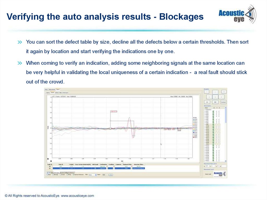
You can sort the defect table by size, decline all the defects below a certain thresholds. Then sortit again by location and start verifying the indications one by one.
When coming to verify an indication, adding some neighboring signals at the same location can
be very helpful in validating the local uniqueness of a certain indication - a real fault should stick
out of the crowd.
14. Verifying the auto analysis results - Erosions
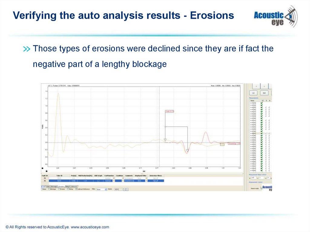
Those types of erosions were declined since they are if fact thenegative part of a lengthy blockage
15. Verifying the auto analysis results - Pitting
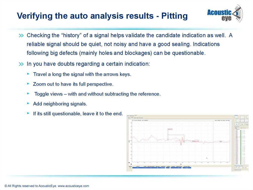
Checking the “history” of a signal helps validate the candidate indication as well. Areliable signal should be quiet, not noisy and have a good sealing. Indications
following big defects (mainly holes and blockages) can be questionable.
In you have doubts regarding a certain indication:
• Travel a long the signal with the arrows keys.
• Zoom out to have its full perspective.
• Toggle views – with and without subtracting the reference.
• Add neighboring signals.
• If its still questionable, leave it to the end.
16. Quick Full Manual Verification
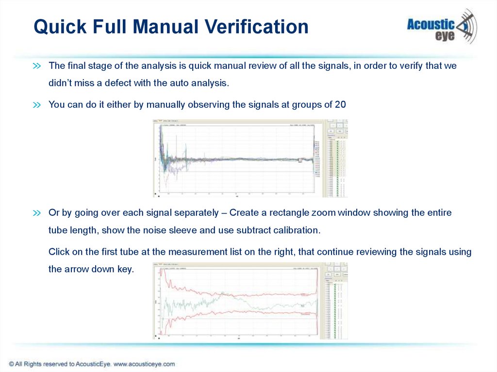
The final stage of the analysis is quick manual review of all the signals, in order to verify that wedidn’t miss a defect with the auto analysis.
You can do it either by manually observing the signals at groups of 20
Or by going over each signal separately – Create a rectangle zoom window showing the entire
tube length, show the noise sleeve and use subtract calibration.
Click on the first tube at the measurement list on the right, that continue reviewing the signals using
the arrow down key.
17. Miscellaneous – Filters Usage
Different types of defects live in different frequency range.• Blockages, Pitting and Erosion are enhanced at high frequency.
• Holes are enhanced at low frequency.
The APR signal is a wide band pulse containing lower and higher frequencies. The auto-analysis
apply different filters in order to detect the different types.
“Detection filter” is the filter at which the defect was detected.
“Display filter” enable the user 5 different filtering options
When applying a certain filter, all relevant display data gets
Updated – thresholds, theoretical signatures.
Examples for filter usages:
• Filtering external noise in order to ease the manual verification.
• Detection enhancement – When the system reported a defect that can’t be easily verified using the
“none” filter.
Toggle to the filter at which the defect was detected. after verifying it’s existence, switch to the”none”
filter in order to classify it.
18. Miscellaneous – Filters Usage Small Pitting Detection
Using the “None” filter:Using the “high_bp” filter:
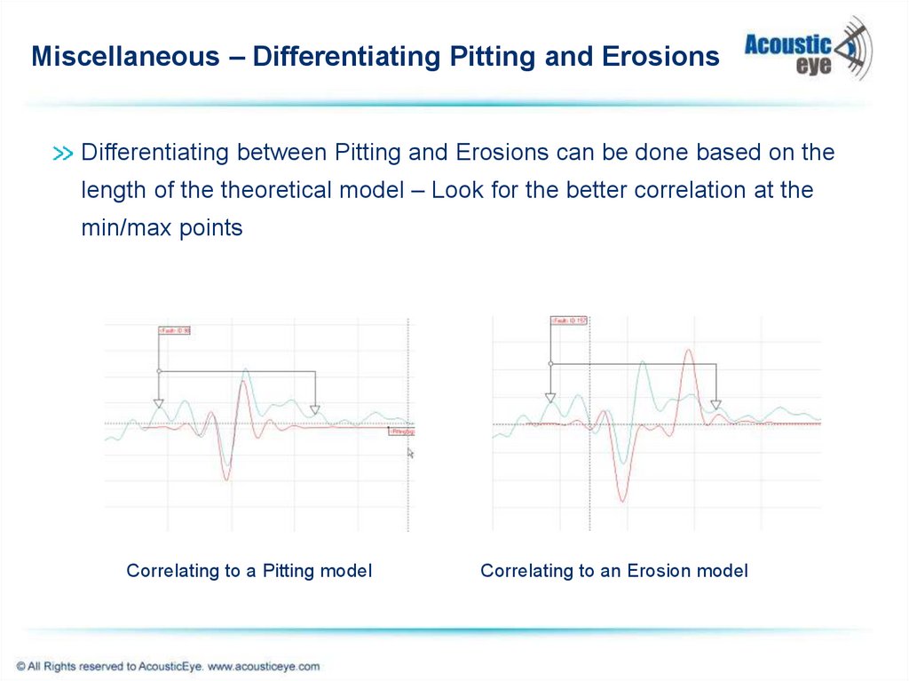
19. Miscellaneous – Differentiating Pitting and Erosions
Differentiating between Pitting and Erosions can be done based on thelength of the theoretical model – Look for the better correlation at the
min/max points
Correlating to a Pitting model
Correlating to an Erosion model



 Электроника


