Chapter 24. Portfolio performance evaluation

1.

CHAPTER 24
Portfolio Performance Evaluation
INVESTMENTS | BODIE, KANE, MARCUS
McGraw-Hill/Irwin
Copyright © 2011 by The McGraw-Hill Companies, Inc. All rights reserved.

2.

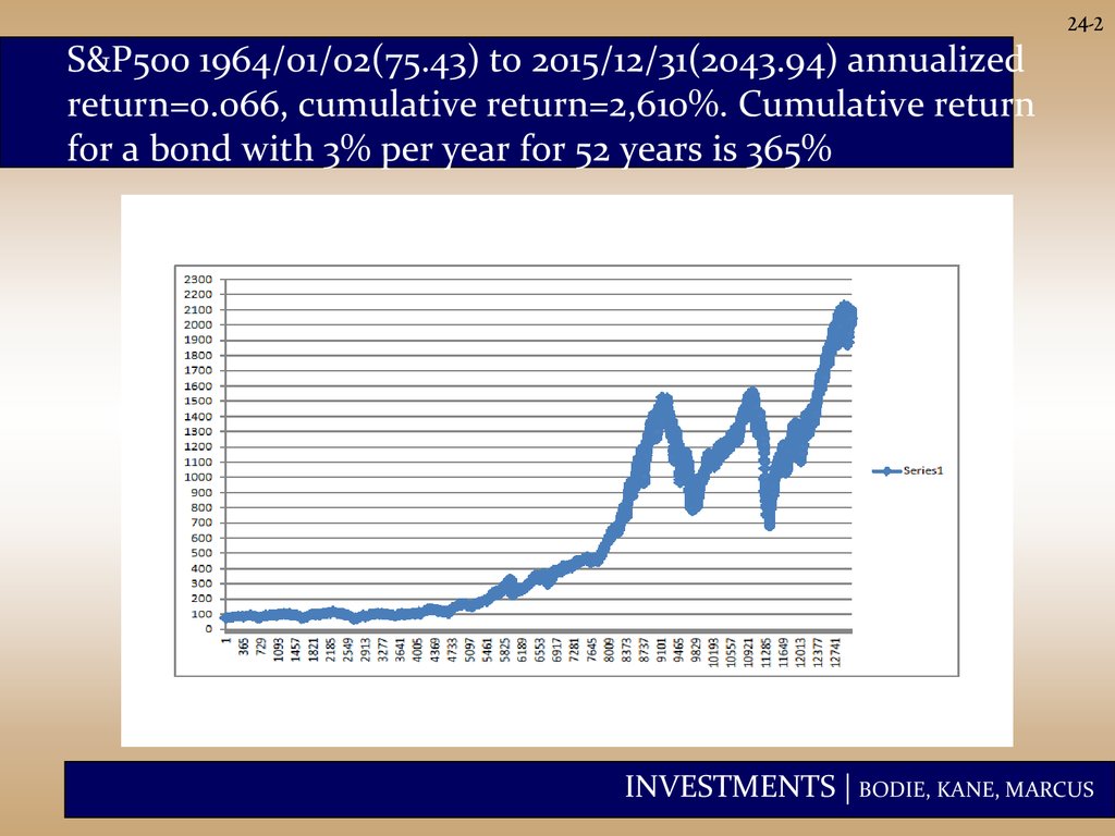
24-2
S&P500 1964/01/02(75.43) to 2015/12/31(2043.94) annualized
return=0.066, cumulative return=2,610%. Cumulative return
for a bond with 3% per year for 52 years is 365%
INVESTMENTS | BODIE, KANE, MARCUS

3.

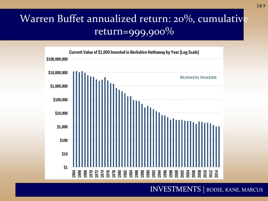
24-3
Warren Buffet annualized return: 20%, cumulative
return=999,900%
INVESTMENTS | BODIE, KANE, MARCUS

4.

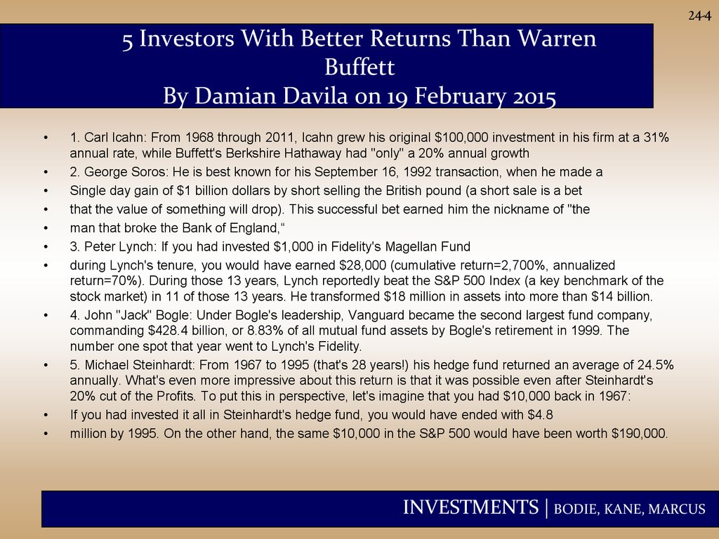
24-4
5 Investors With Better Returns Than Warren
Buffett
By Damian Davila on 19 February 2015
1. Carl Icahn: From 1968 through 2011, Icahn grew his original $100,000 investment in his firm at a 31%
annual rate, while Buffett's Berkshire Hathaway had "only" a 20% annual growth
2. George Soros: He is best known for his September 16, 1992 transaction, when he made a
Single day gain of $1 billion dollars by short selling the British pound (a short sale is a bet
that the value of something will drop). This successful bet earned him the nickname of "the
man that broke the Bank of England,“
3. Peter Lynch: If you had invested $1,000 in Fidelity's Magellan Fund
during Lynch's tenure, you would have earned $28,000 (cumulative return=2,700%, annualized
return=70%). During those 13 years, Lynch reportedly beat the S&P 500 Index (a key benchmark of the
stock market) in 11 of those 13 years. He transformed $18 million in assets into more than $14 billion.
4. John "Jack" Bogle: Under Bogle's leadership, Vanguard became the second largest fund company,
commanding $428.4 billion, or 8.83% of all mutual fund assets by Bogle's retirement in 1999. The
number one spot that year went to Lynch's Fidelity.
5. Michael Steinhardt: From 1967 to 1995 (that's 28 years!) his hedge fund returned an average of 24.5%
annually. What's even more impressive about this return is that it was possible even after Steinhardt's
20% cut of the Profits. To put this in perspective, let's imagine that you had $10,000 back in 1967:
If you had invested it all in Steinhardt's hedge fund, you would have ended with $4.8
million by 1995. On the other hand, the same $10,000 in the S&P 500 would have been worth $190,000.
INVESTMENTS | BODIE, KANE, MARCUS

5.

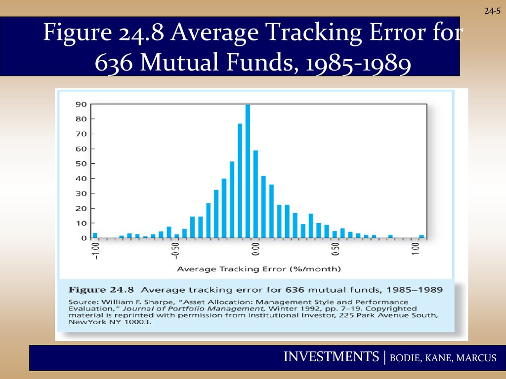
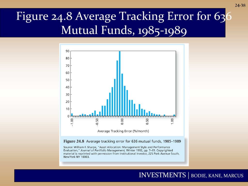
24-5
Figure 24.8 Average Tracking Error for
636 Mutual Funds, 1985-1989
INVESTMENTS | BODIE, KANE, MARCUS

6.

24-6
Introduction
• Two common ways to measure
average portfolio return:
1. Time-weighted returns
2. Dollar-weighted returns
• Returns must be adjusted for risk.
INVESTMENTS | BODIE, KANE, MARCUS

7.

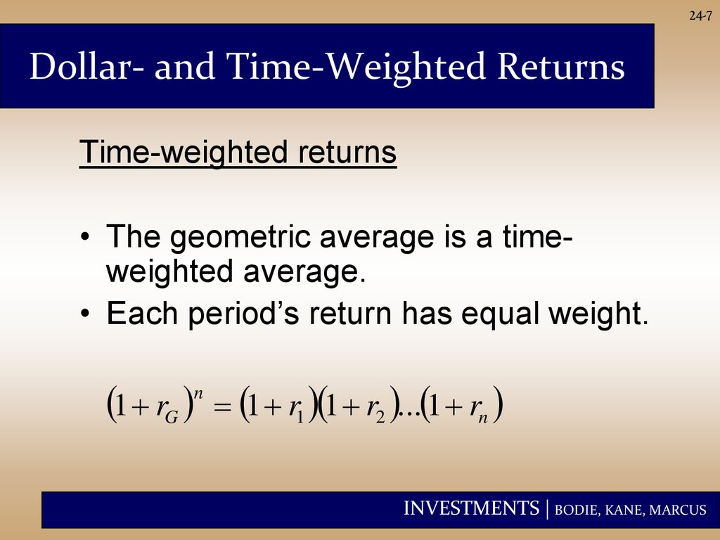
24-7
Dollar- and Time-Weighted Returns
Time-weighted returns
• The geometric average is a timeweighted average.
• Each period’s return has equal weight.
1 rG
n
1 r1 1 r2 ... 1 rn
INVESTMENTS | BODIE, KANE, MARCUS

8.

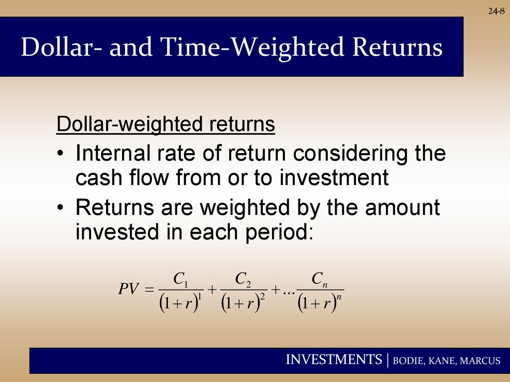
24-8
Dollar- and Time-Weighted Returns
Dollar-weighted returns
• Internal rate of return considering the
cash flow from or to investment
• Returns are weighted by the amount
invested in each period:
PV
Cn
C1
C2
...
1 r 1 1 r 2 1 r n
INVESTMENTS | BODIE, KANE, MARCUS

9.

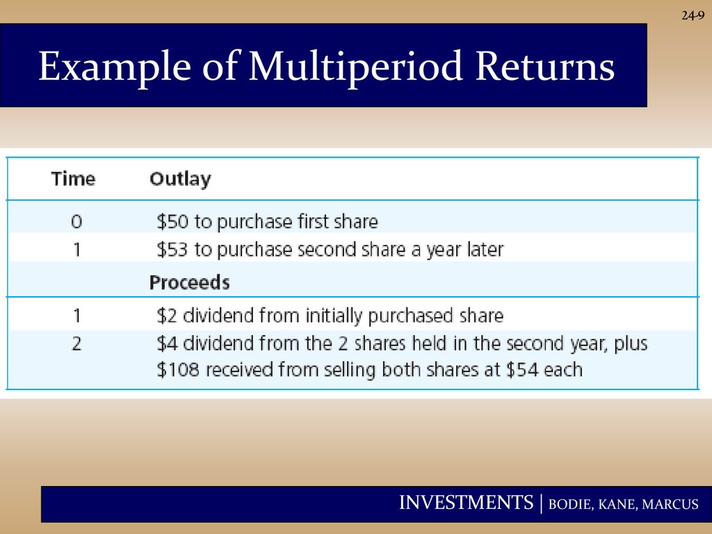
24-9
Example of Multiperiod Returns
INVESTMENTS | BODIE, KANE, MARCUS

10.

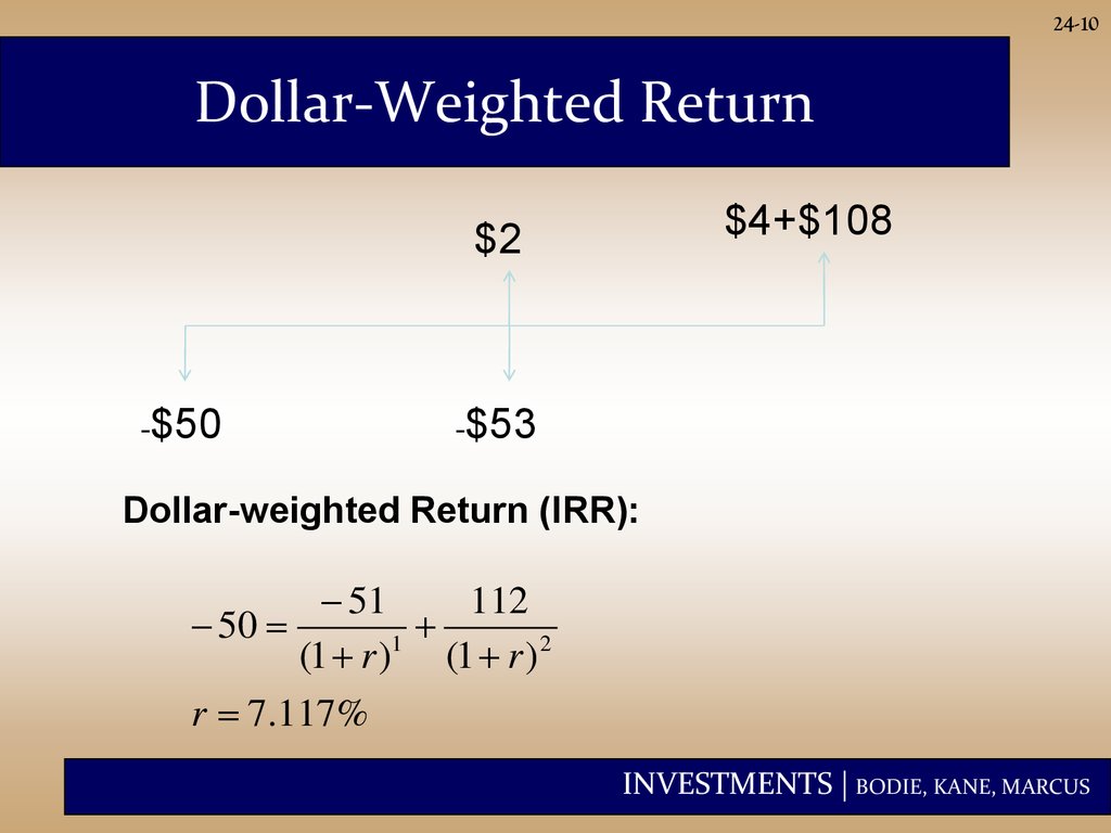
24-10
Dollar-Weighted Return
$4+$108
$2
-$50
-$53
Dollar-weighted Return (IRR):
51
112
50
1
(1 r ) (1 r ) 2
r 7.117%
INVESTMENTS | BODIE, KANE, MARCUS

11.

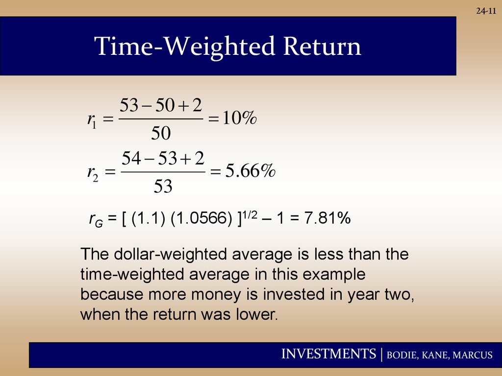
24-11
Time-Weighted Return
53 50 2
r1
10%
50
54 53 2
r2
5.66%
53
rG = [ (1.1) (1.0566) ]1/2 – 1 = 7.81%
The dollar-weighted average is less than the
time-weighted average in this example
because more money is invested in year two,
when the return was lower.
INVESTMENTS | BODIE, KANE, MARCUS

12.

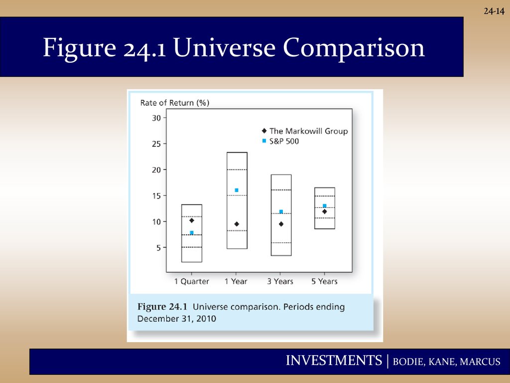
24-12
Adjusting Returns for Risk
• The simplest and most popular way to
adjust returns for risk is to compare
the portfolio’s return with the returns
on a comparison universe.
• The comparison universe is a
benchmark composed of a group of
funds or portfolios with similar risk
characteristics, such as growth stock
funds or high-yield bond funds.
INVESTMENTS | BODIE, KANE, MARCUS

13.

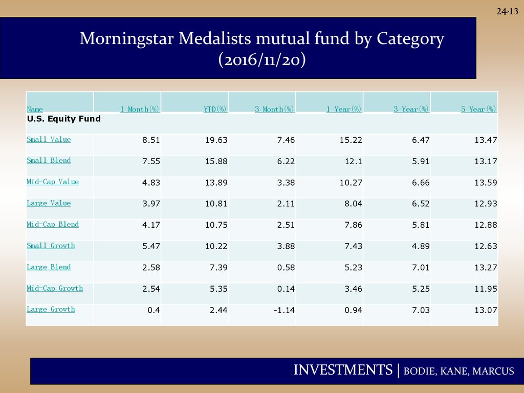
24-13
Morningstar Medalists mutual fund by Category
(2016/11/20)
Name
U.S. Equity Fund
1 Month(%)
YTD(%)
3 Month(%)
1 Year(%)
3 Year(%)
5 Year(%)
Small Value
8.51
19.63
7.46
15.22
6.47
13.47
Small Blend
7.55
15.88
6.22
12.1
5.91
13.17
Mid-Cap Value
4.83
13.89
3.38
10.27
6.66
13.59
Large Value
3.97
10.81
2.11
8.04
6.52
12.93
Mid-Cap Blend
4.17
10.75
2.51
7.86
5.81
12.88
Small Growth
5.47
10.22
3.88
7.43
4.89
12.63
Large Blend
2.58
7.39
0.58
5.23
7.01
13.27
Mid-Cap Growth
2.54
5.35
0.14
3.46
5.25
11.95
0.4
2.44
-1.14
0.94
7.03
13.07
Large Growth
INVESTMENTS | BODIE, KANE, MARCUS

14.

24-14
Figure 24.1 Universe Comparison
INVESTMENTS | BODIE, KANE, MARCUS

15.

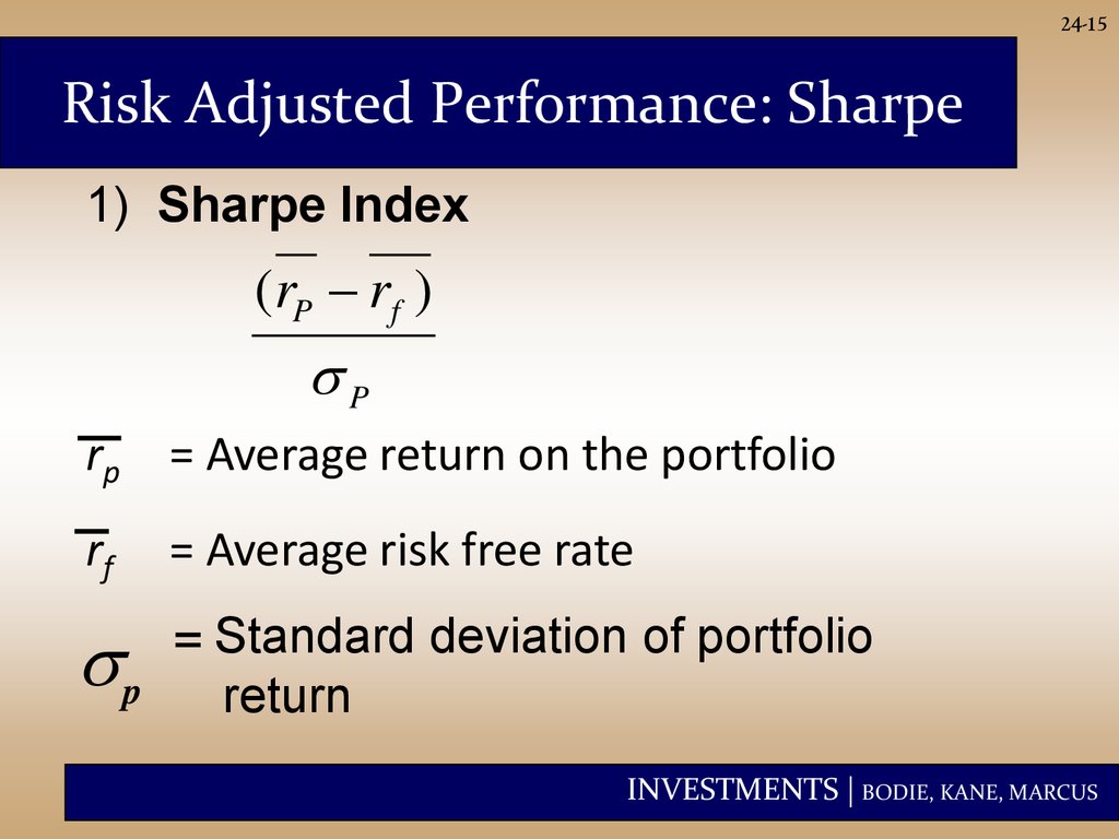
24-15
Risk Adjusted Performance: Sharpe
1) Sharpe Index
(rP rf )
P
rp = Average return on the portfolio
rf
= Average risk free rate
p
= Standard deviation of portfolio
return
INVESTMENTS | BODIE, KANE, MARCUS

16.

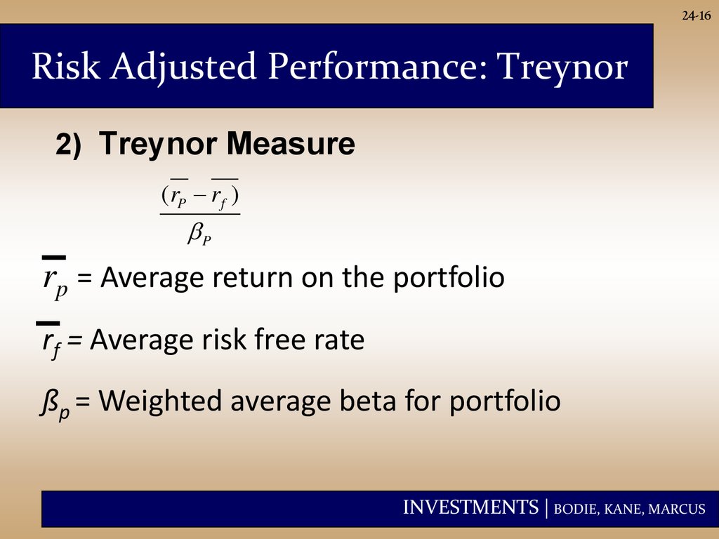
24-16
Risk Adjusted Performance: Treynor
2) Treynor Measure
(rP rf )
P
rp = Average return on the portfolio
rf = Average risk free rate
ßp = Weighted average beta for portfolio
INVESTMENTS | BODIE, KANE, MARCUS

17.

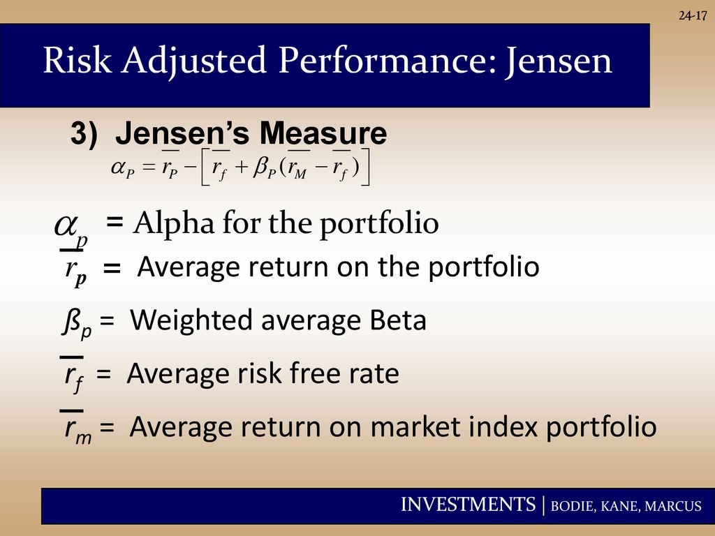
24-17
Risk Adjusted Performance: Jensen
3) Jensen’s Measure
P rP rf P (rM rf )
p
= Alpha for the portfolio
rp = Average return on the portfolio
ßp = Weighted average Beta
rf = Average risk free rate
rm = Average return on market index portfolio
INVESTMENTS | BODIE, KANE, MARCUS

18.

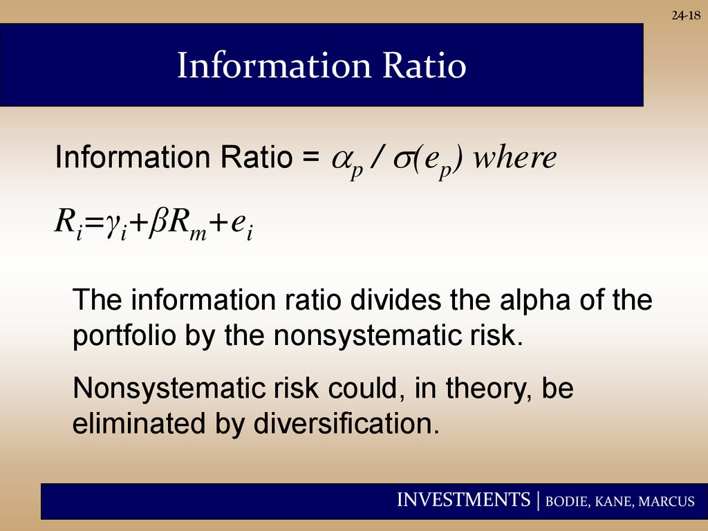
24-18
Information Ratio
Information Ratio = p / (ep) where
Ri=γi+βRm+ei
The information ratio divides the alpha of the
portfolio by the nonsystematic risk.
Nonsystematic risk could, in theory, be
eliminated by diversification.
INVESTMENTS | BODIE, KANE, MARCUS

19.

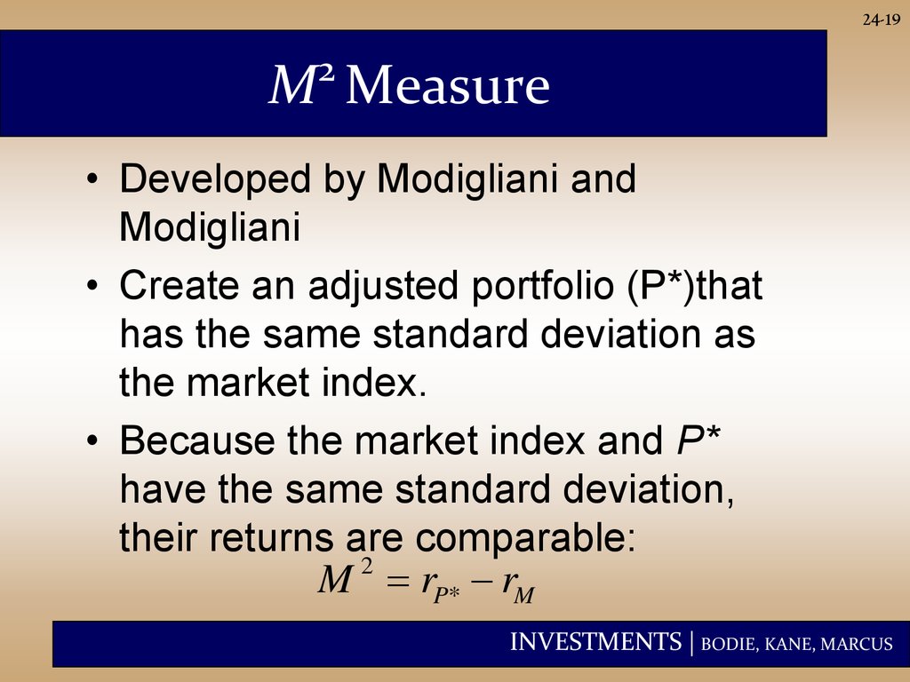
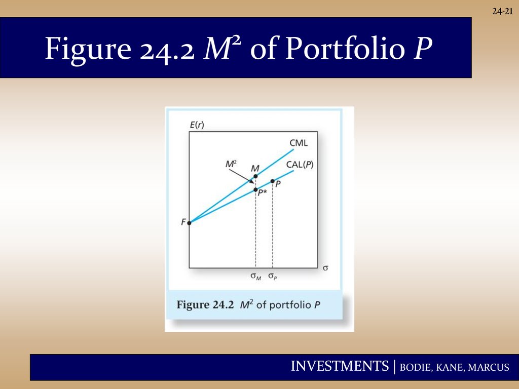
24-19
2
M Measure
• Developed by Modigliani and
Modigliani
• Create an adjusted portfolio (P*)that
has the same standard deviation as
the market index.
• Because the market index and P*
have the same standard deviation,
their returns are comparable:
2
M rP* rM
INVESTMENTS | BODIE, KANE, MARCUS

20.

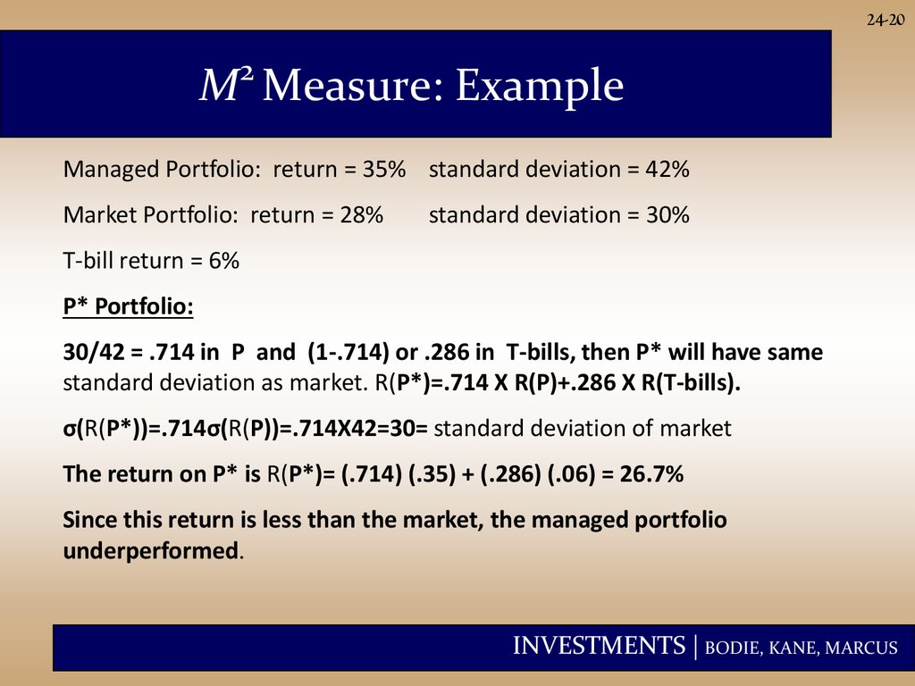
24-20
2
M Measure: Example
Managed Portfolio: return = 35% standard deviation = 42%
Market Portfolio: return = 28%
standard deviation = 30%
T-bill return = 6%
P* Portfolio:
30/42 = .714 in P and (1-.714) or .286 in T-bills, then P* will have same
standard deviation as market. R(P*)=.714 X R(P)+.286 X R(T-bills).
σ(R(P*))=.714σ(R(P))=.714X42=30= standard deviation of market
The return on P* is R(P*)= (.714) (.35) + (.286) (.06) = 26.7%
Since this return is less than the market, the managed portfolio
underperformed.
INVESTMENTS | BODIE, KANE, MARCUS

21.

24-21
2
Figure 24.2 M of Portfolio P
INVESTMENTS | BODIE, KANE, MARCUS

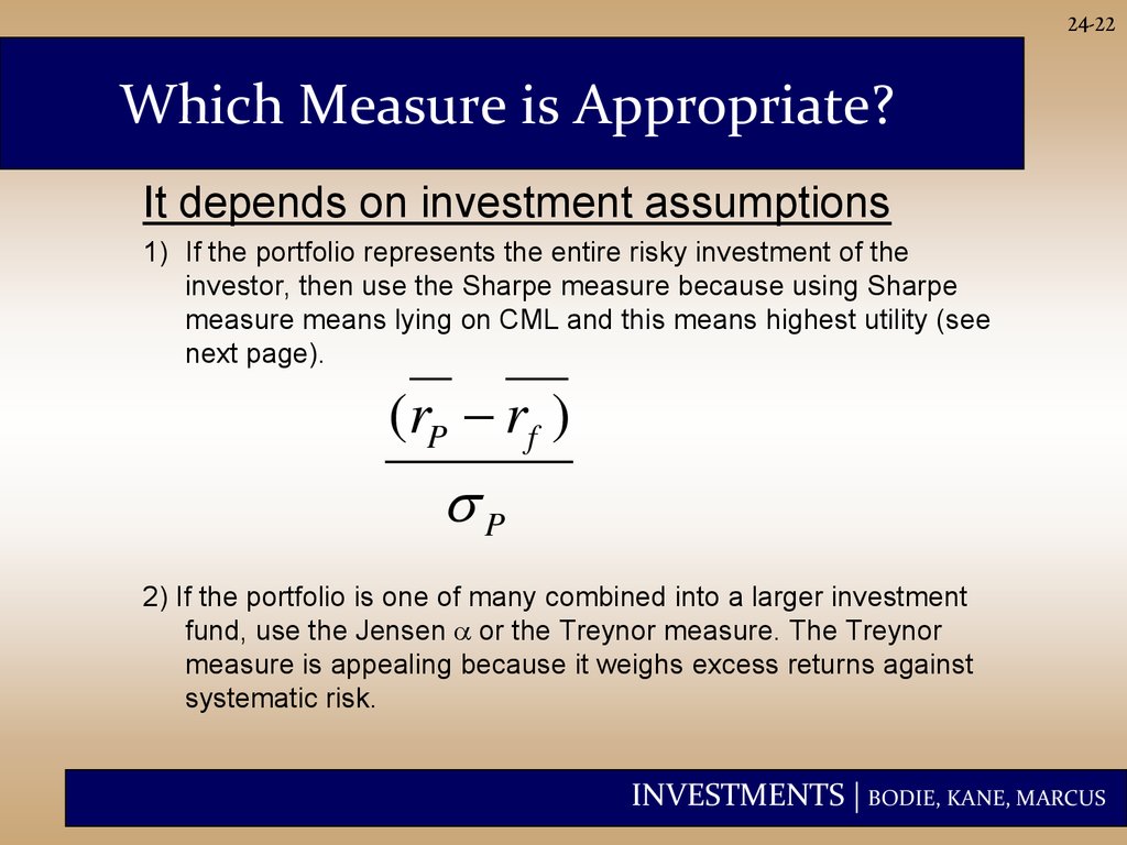
22.

24-22
Which Measure is Appropriate?
It depends on investment assumptions
1) If the portfolio represents the entire risky investment of the
investor, then use the Sharpe measure because using Sharpe
measure means lying on CML and this means highest utility (see
next page).
(rP rf )
P
2) If the portfolio is one of many combined into a larger investment
fund, use the Jensen or the Treynor measure. The Treynor
measure is appealing because it weighs excess returns against
systematic risk.
INVESTMENTS | BODIE, KANE, MARCUS

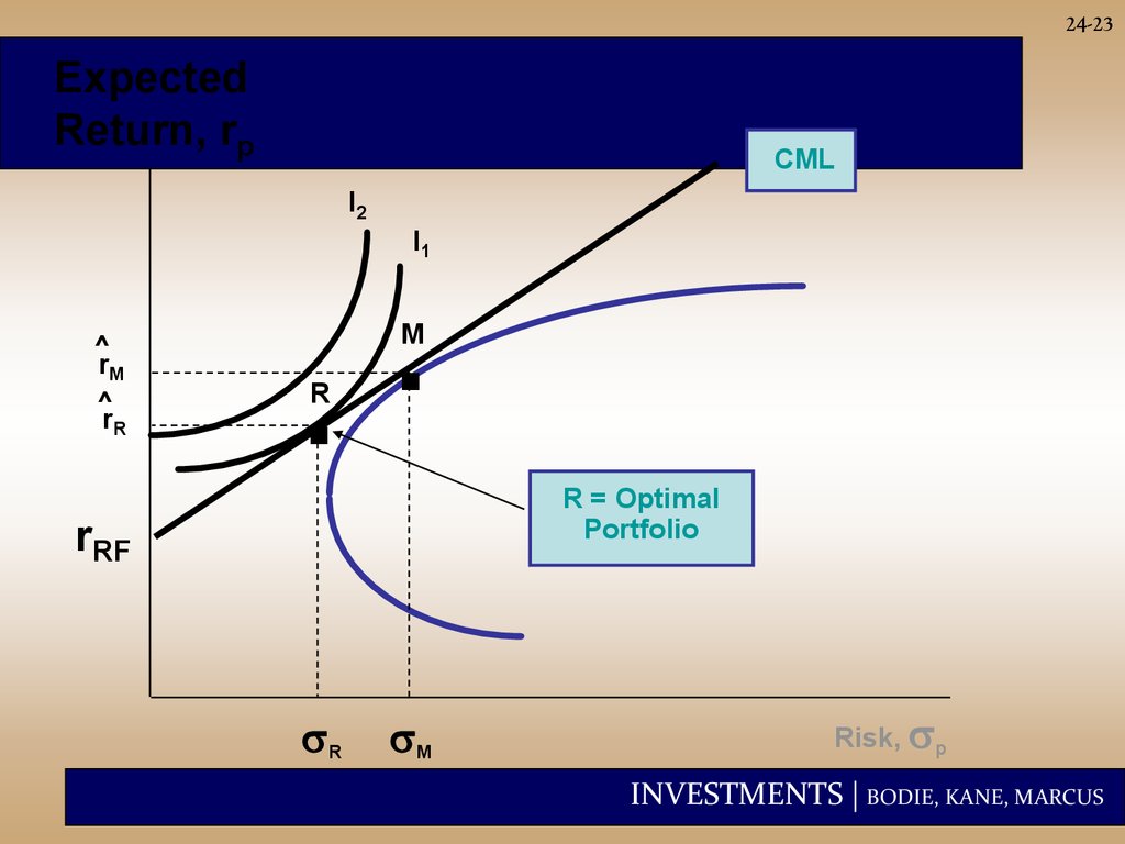
23.

24-23
Expected
Return, rp
CML
I2
I1
^
rM
^
rR
.
.
M
R
R = Optimal
Portfolio
rRF
R
M
Risk, p
INVESTMENTS | BODIE, KANE, MARCUS

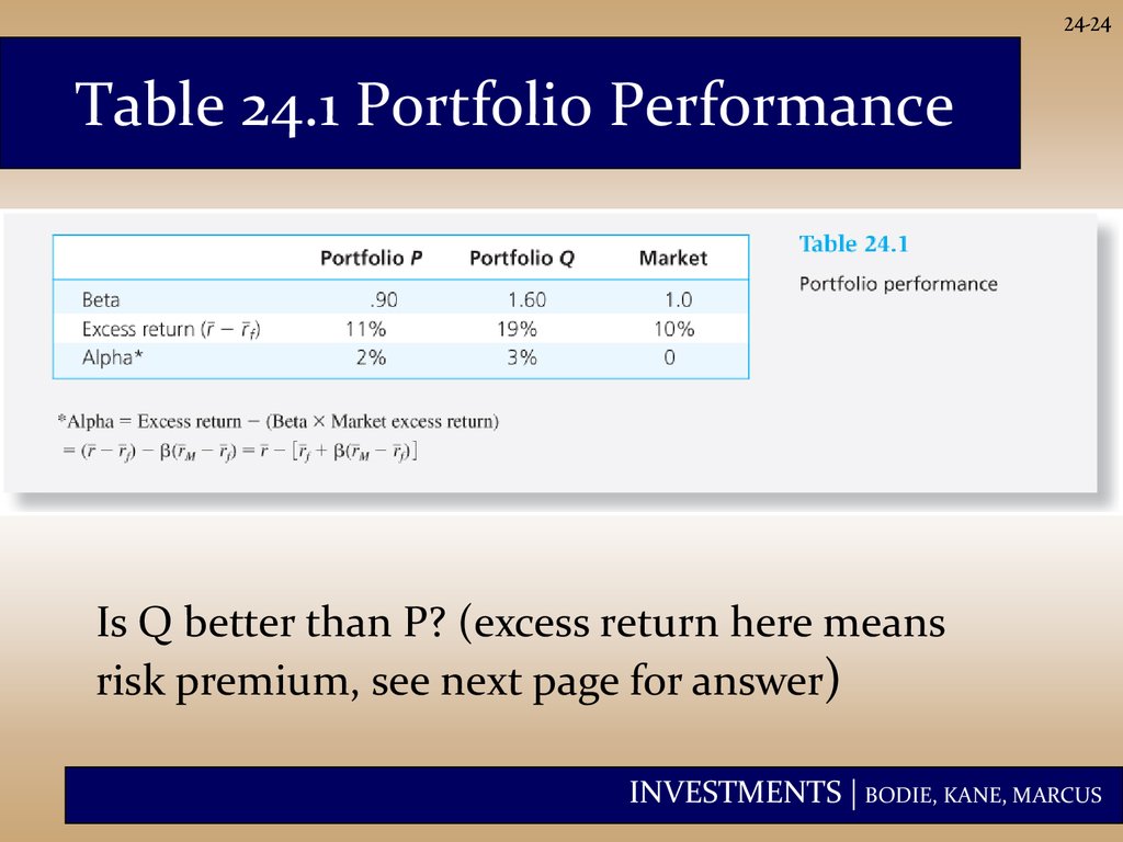
24.

24-24
Table 24.1 Portfolio Performance
Is Q better than P? (excess return here means
risk premium, see next page for answer)
INVESTMENTS | BODIE, KANE, MARCUS

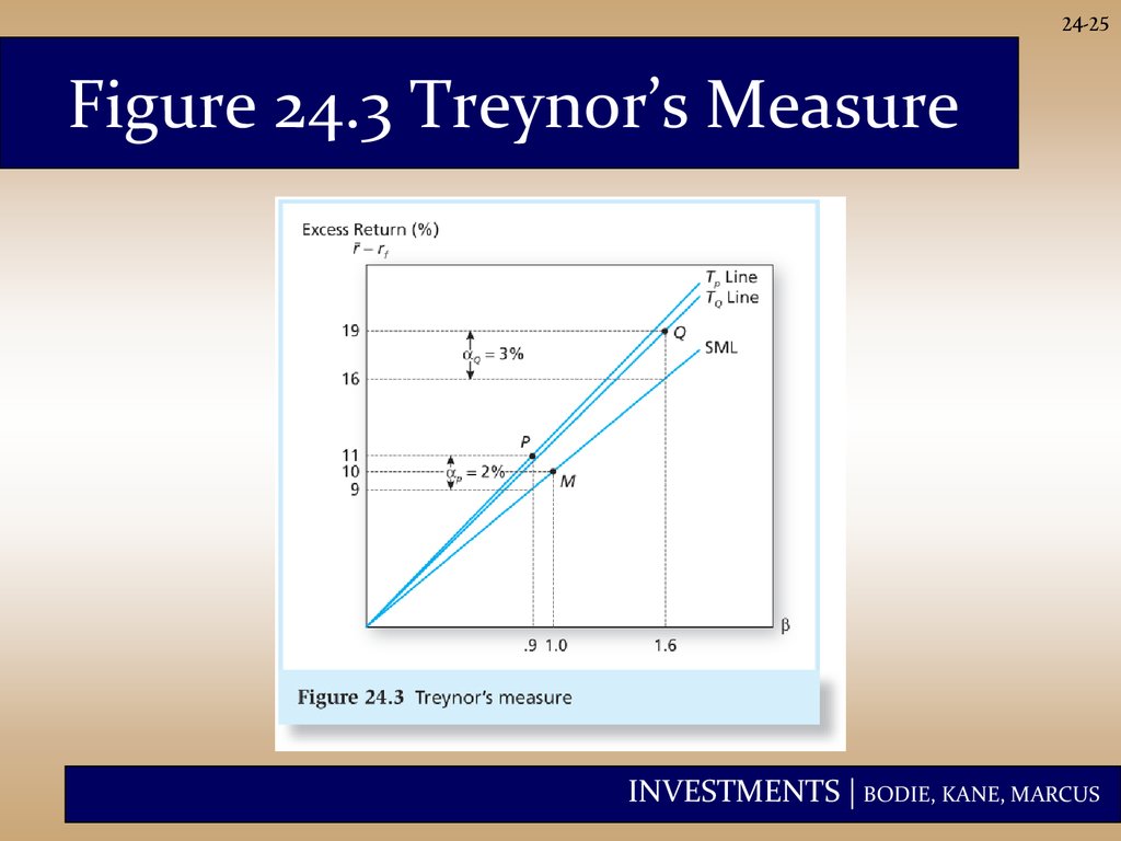
25.

24-25
Figure 24.3 Treynor’s Measure
INVESTMENTS | BODIE, KANE, MARCUS

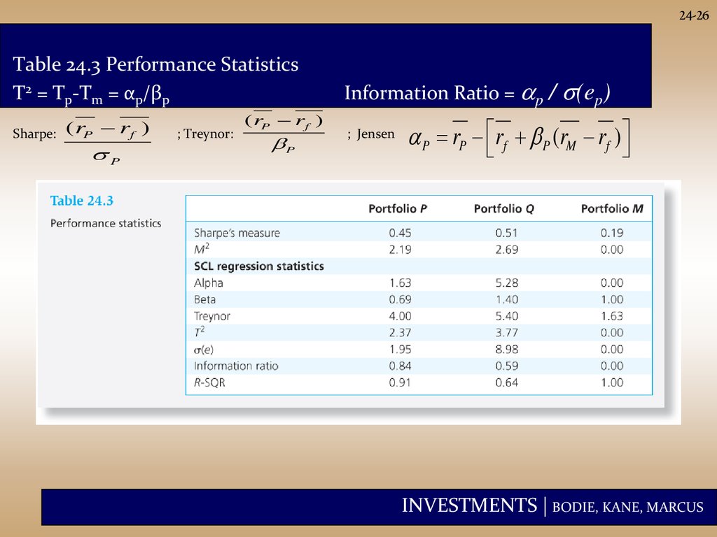
26.

24-26
Table 24.3 Performance Statistics
T2 = Tp-Tm = αp/βp
Sharpe:
( rP rf )
P
; Treynor:
( rP rf )
P
Information Ratio = p /
; Jensen
(ep)
P rP rf P (rM rf )
INVESTMENTS | BODIE, KANE, MARCUS

27.

24-27
Interpretation of Table 24.3
• If P or Q represents the entire investment, Q
is better because of its higher Sharpe
measure and better M2.
• If P and Q are competing for a role as one of
a number of subportfolios, Q also dominates
because its Treynor measure is higher.
• If we seek an active portfolio to mix with an
index portfolio, P is better due to its higher
information ratio. (explanation next page)
INVESTMENTS | BODIE, KANE, MARCUS

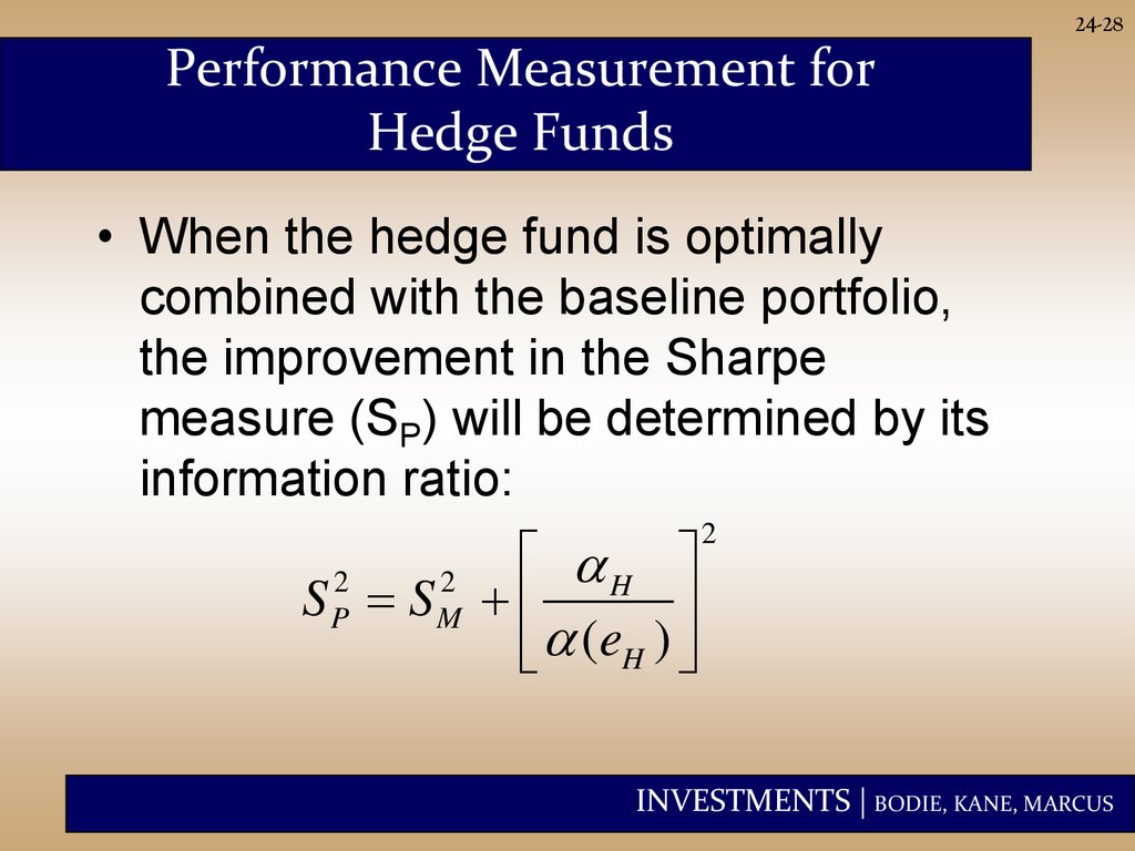
28.

24-28
Performance Measurement for
Hedge Funds
• When the hedge fund is optimally
combined with the baseline portfolio,
the improvement in the Sharpe
measure (SP) will be determined by its
information ratio:
H
S S
(eH )
2
P
2
2
M
INVESTMENTS | BODIE, KANE, MARCUS

29.

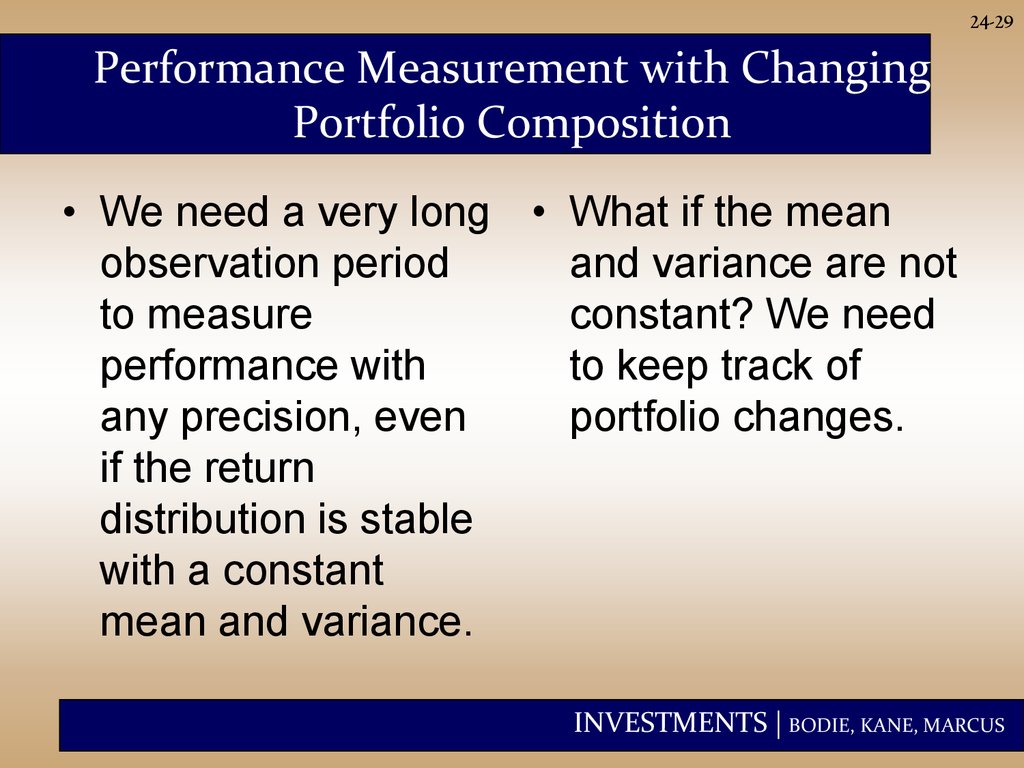
24-29
Performance Measurement with Changing
Portfolio Composition
• We need a very long • What if the mean
observation period
and variance are not
to measure
constant? We need
performance with
to keep track of
any precision, even
portfolio changes.
if the return
distribution is stable
with a constant
mean and variance.
INVESTMENTS | BODIE, KANE, MARCUS

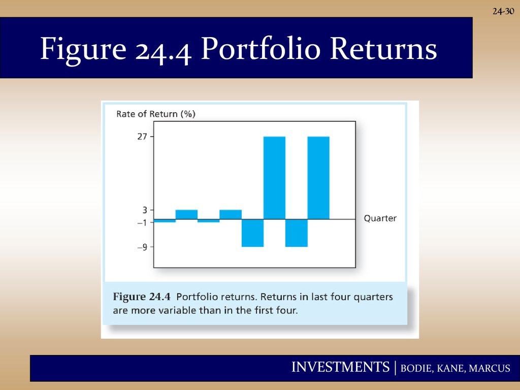
30.

24-30
Figure 24.4 Portfolio Returns
INVESTMENTS | BODIE, KANE, MARCUS

31.

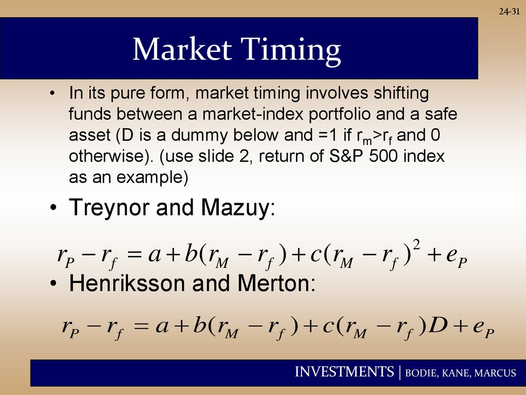
24-31
Market Timing
• In its pure form, market timing involves shifting
funds between a market-index portfolio and a safe
asset (D is a dummy below and =1 if rm>rf and 0
otherwise). (use slide 2, return of S&P 500 index
as an example)
• Treynor and Mazuy:
rP rf a b(rM rf ) c(rM rf ) eP
2
• Henriksson and Merton:
rP rf a b(rM rf ) c (rM rf ) D eP
INVESTMENTS | BODIE, KANE, MARCUS

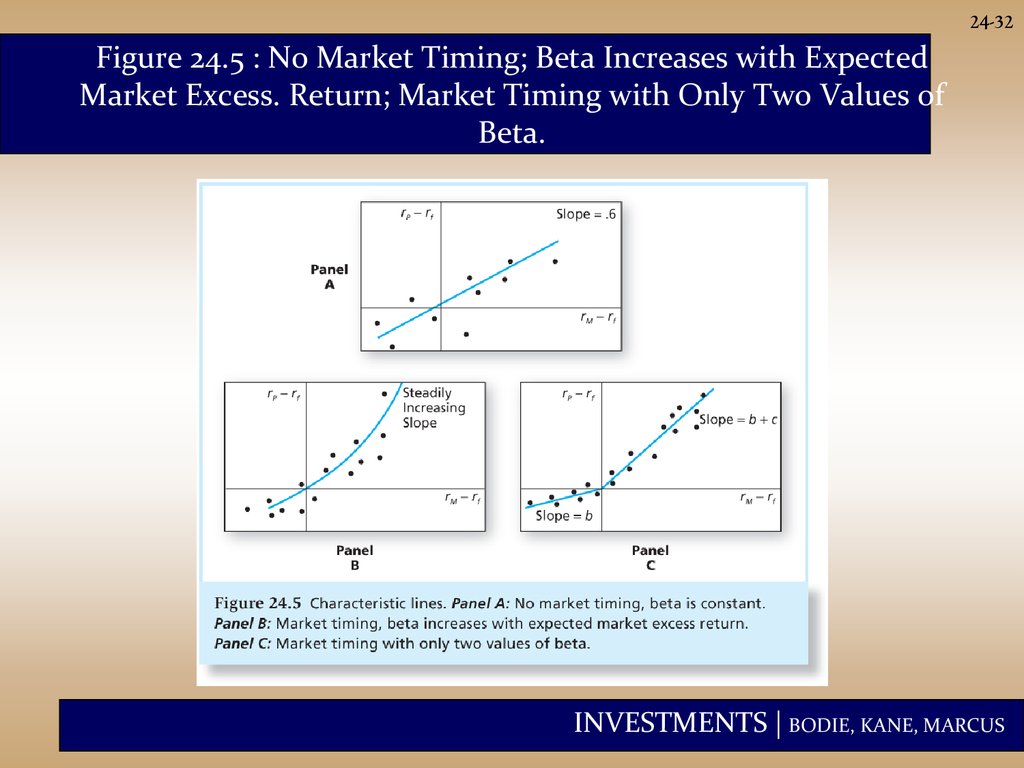
32.

24-32
Figure 24.5 : No Market Timing; Beta Increases with Expected
Market Excess. Return; Market Timing with Only Two Values of
Beta.
INVESTMENTS | BODIE, KANE, MARCUS

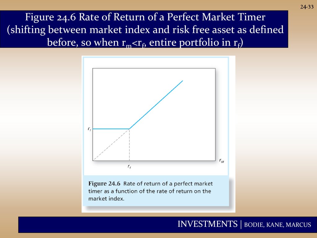
33.

24-33
Figure 24.6 Rate of Return of a Perfect Market Timer
(shifting between market index and risk free asset as defined
before, so when rm<rf, entire portfolio in rf)
INVESTMENTS | BODIE, KANE, MARCUS

34.

24-34
Style Analysis
• Introduced by William Sharpe
• Regress fund returns on indexes representing a
range of asset classes.
• R(index)=α+β1Xasset class 1+ β2Xasset class 2 +… +error
• The regression coefficient on each index
measures the fund’s implicit allocation to that
“style.”
• R –square measures return variability due to style
or asset allocation.
• The remainder is due either to security selection
or to market timing.
INVESTMENTS | BODIE, KANE, MARCUS

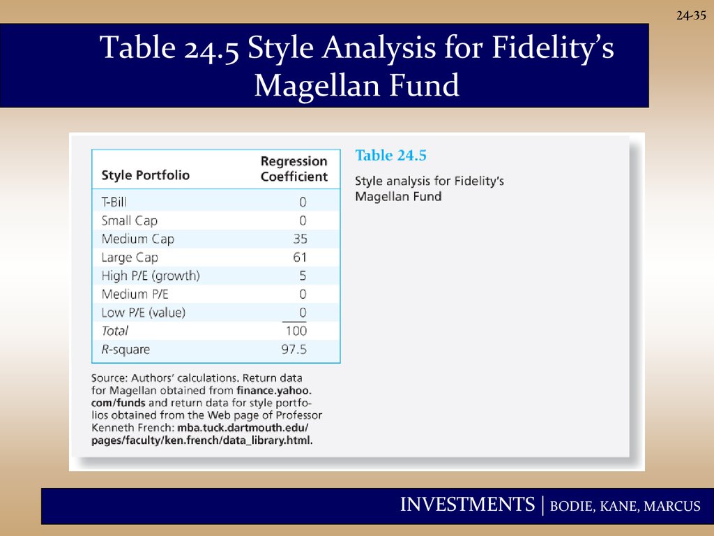
35.

24-35
Table 24.5 Style Analysis for Fidelity’s
Magellan Fund
INVESTMENTS | BODIE, KANE, MARCUS

36.

24-36
Morningstar Medalists mutual fund by Category
2016/11/20
Name
U.S. Equity Fund
1 Month(%)
YTD(%)
3 Month(%)
1 Year(%)
3 Year(%)
5 Year(%)
Small Value
8.51
19.63
7.46
15.22
6.47
13.47
Small Blend
7.55
15.88
6.22
12.1
5.91
13.17
Mid-Cap Value
4.83
13.89
3.38
10.27
6.66
13.59
Large Value
3.97
10.81
2.11
8.04
6.52
12.93
Mid-Cap Blend
4.17
10.75
2.51
7.86
5.81
12.88
Small Growth
5.47
10.22
3.88
7.43
4.89
12.63
Large Blend
2.58
7.39
0.58
5.23
7.01
13.27
Mid-Cap Growth
2.54
5.35
0.14
3.46
5.25
11.95
0.4
2.44
-1.14
0.94
7.03
13.07
Large Growth
INVESTMENTS | BODIE, KANE, MARCUS

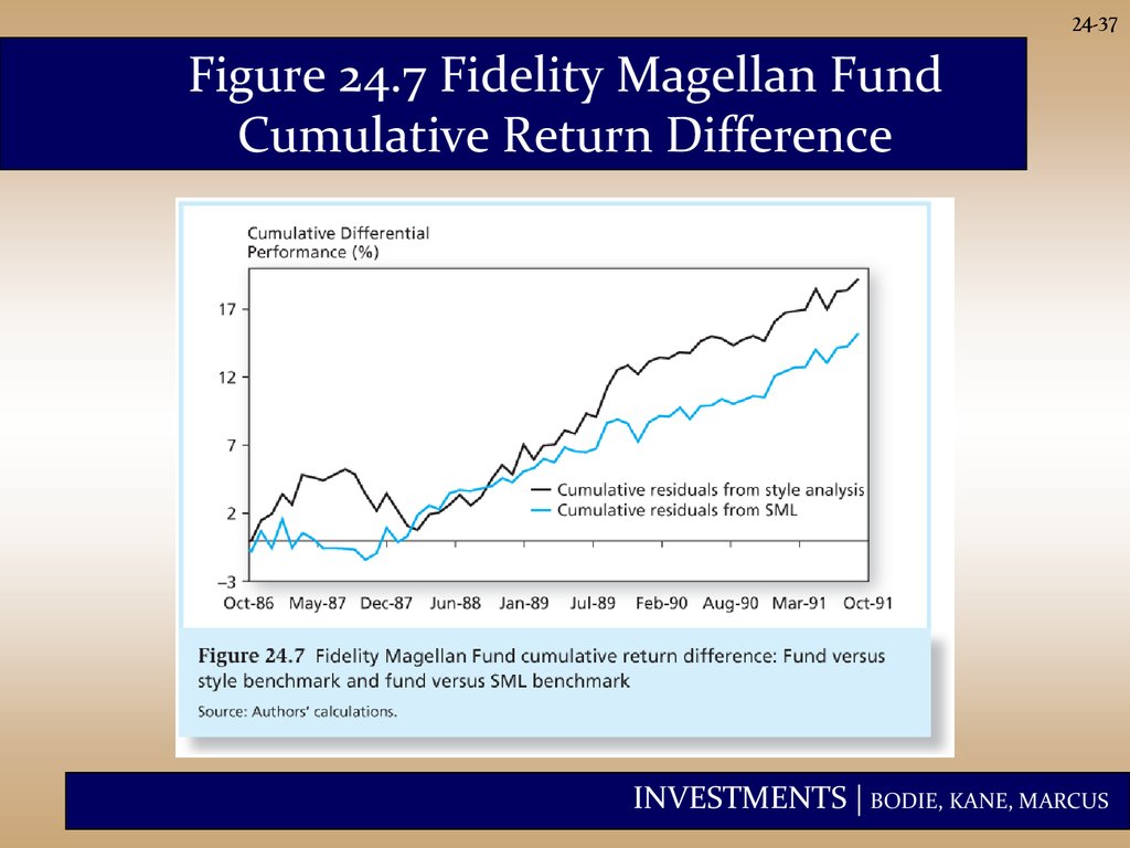
37.

24-37
Figure 24.7 Fidelity Magellan Fund
Cumulative Return Difference
INVESTMENTS | BODIE, KANE, MARCUS

38.

24-38
Figure 24.8 Average Tracking Error for 636
Mutual Funds, 1985-1989
INVESTMENTS | BODIE, KANE, MARCUS

39.

24-39
Evaluating Performance Evaluation
• Performance evaluation has two key
problems:
1. Many observations are needed for
significant results.
2. Shifting parameters when portfolios
are actively managed makes
accurate performance evaluation
all the more elusive.
INVESTMENTS | BODIE, KANE, MARCUS

40.

24-40
Performance Attribution
• A common attribution system decomposes
performance into three components:
1. Allocation choices across broad asset
classes.
2. Industry or sector choice within each
market.
3. Security choice within each sector.
INVESTMENTS | BODIE, KANE, MARCUS

41.

24-41
Attributing Performance to
Components
Set up a ‘Benchmark’ or ‘Bogey’
portfolio:
• Select a benchmark index portfolio for
each asset class.
• Choose weights based on market
expectations.
• Choose a portfolio of securities within
each class by security analysis.
INVESTMENTS | BODIE, KANE, MARCUS

42.

24-42
Attributing Performance to
Components
• Calculate the return on the ‘Bogey’ and on
the managed portfolio.
• Explain the difference in return based on
component weights or selection.
• Summarize the performance differences
into appropriate categories.
INVESTMENTS | BODIE, KANE, MARCUS

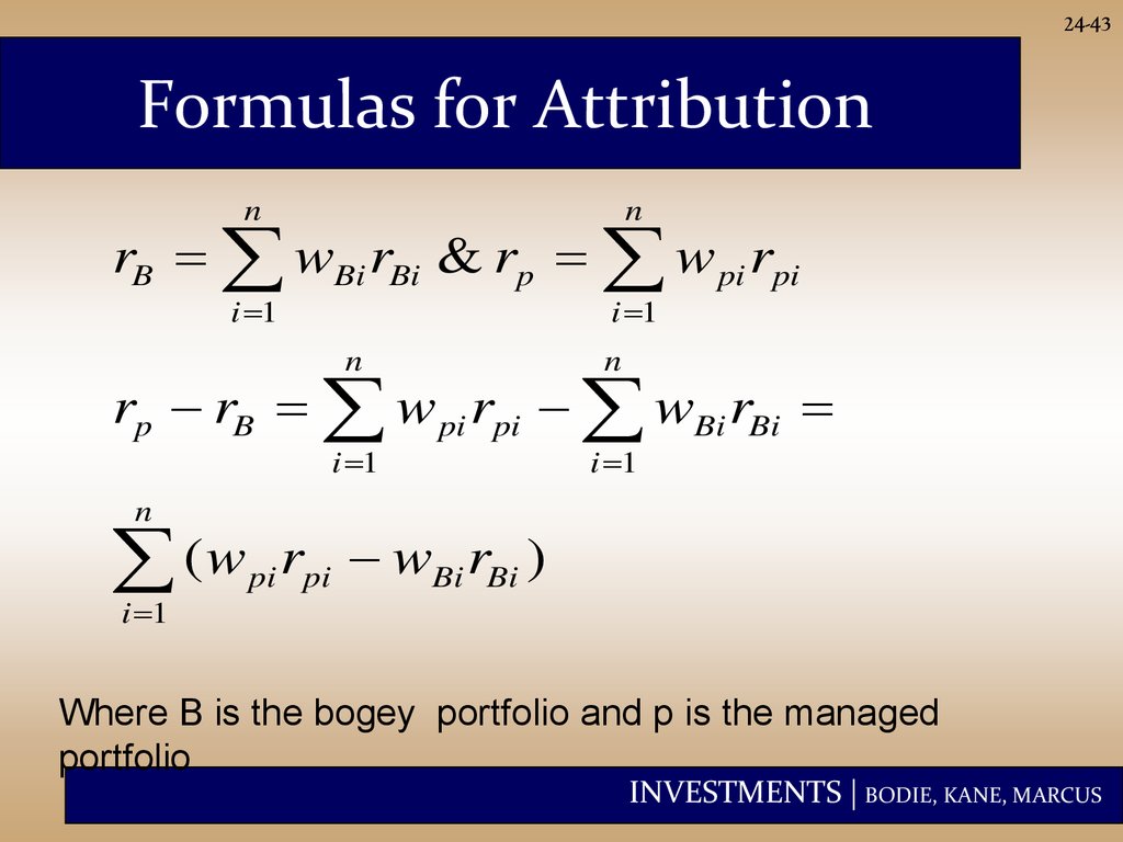
43.

24-43
Formulas for Attribution
n
n
i 1
i 1
rB wBi rBi & rp w pi rpi
n
n
i 1
i 1
rp rB w pi rpi wBi rBi
n
(w
i 1
r wBi rBi )
pi pi
Where B is the bogey portfolio and p is the managed
portfolio
INVESTMENTS | BODIE, KANE, MARCUS

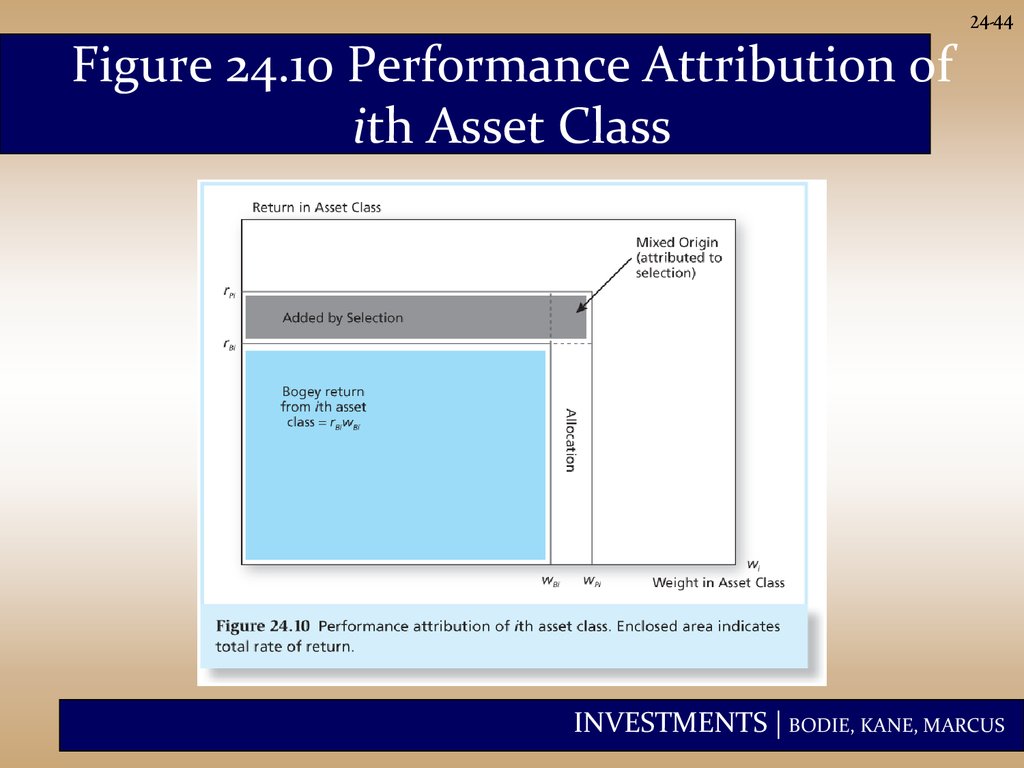
44.

24-44
Figure 24.10 Performance Attribution of
ith Asset Class
INVESTMENTS | BODIE, KANE, MARCUS

45.

24-45
Performance Attribution
• Superior performance is achieved by:
– overweighting assets in markets that
perform well
– underweighting assets in poorly
performing markets
INVESTMENTS | BODIE, KANE, MARCUS

46.

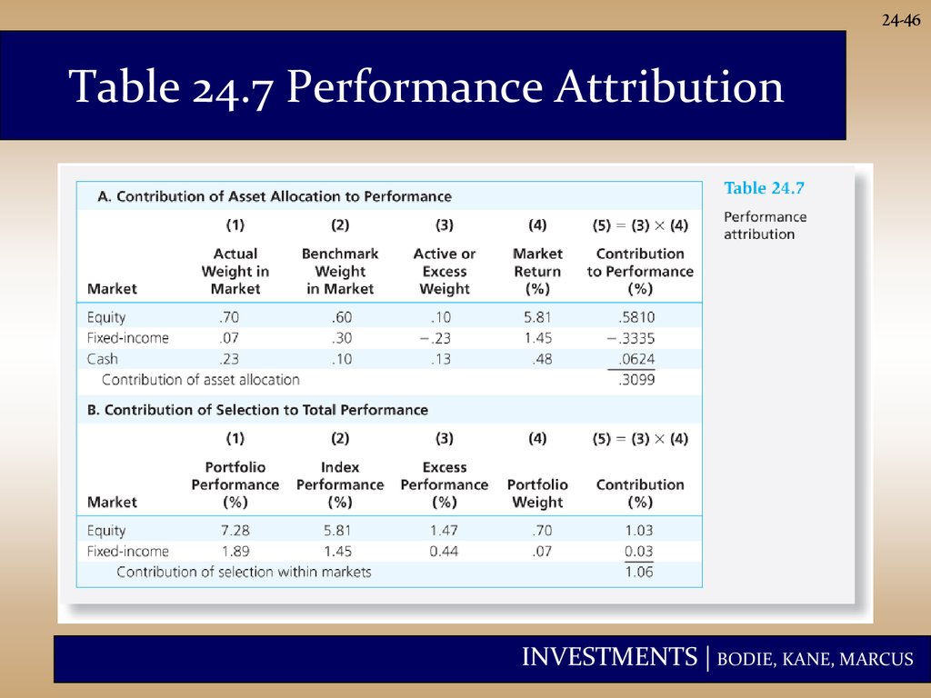
24-46
Table 24.7 Performance Attribution
INVESTMENTS | BODIE, KANE, MARCUS

47.

24-47
Sector and Security Selection
• Good performance
(a positive
contribution)
derives from
overweighting
high-performing
sectors
• Good performance
also derives from
underweighting
poorly performing
sectors.
INVESTMENTS | BODIE, KANE, MARCUS