Set of realizations – ensemble estimates

Probability density function – PDF (funkce hustoty rozdělení pravděpodobnosti)

Joint probability or joint probability density function

Principle - counting in two different times

Estimating joint probabilities P(Xi , Xj , ni , nj) for discrete data

Continuous range – joint probability density function

Example of joint PDF estimation for water

Variance (dispersion, variance, rozptyl)

Just select data and use formulas known from high school !

Correlation coefficient (korelační koeficient)

Direct ensemble estimate of correlation coefficient

Just select data and multiply the two samples in each realization + normalize

We can even do temporal estimates of joint probabilities !

2.87M

Категории: $Математика$ Математика

Физика

Random signals

1. Random signals

Honza Černocký, ÚPGM
Please open Python notebook random_1

2. Agenda

• Introduction, terminology and data for the rest of this lecture
• Functions describing random signals - CDF, probabilities, and PDF
• Relation between two times - joint probabilities and joint PDF
• Moments - mean and variance
• Correlation coefficients
• Stationarity
• Ergodicity and temporal estimates
• Summary and todo's
2 / 72

3. Signals at school and in the real world

Deterministic
• Equation
• Plot
• Algorithm
• Piece of code
}
Can compute
Little information !
Random
• Don’t know for sure
• All different
• Primarily for „nature“
and „biological“
signals
• Can estimate
parameters
3

4. Examples

• Speech
• Music
• Video
• Currency exchange rates
• Technical signals (diagnostics)
• Measurements (of anything)
• … almost everything
4

5. Mathematically

• Discrete-time only (samples) – we won’t deal with continuous-time
random signals in ISS.
• A system of random variables defined for each n
• For the moment, will look at each time independently
...
5

6. Set of realizations – ensemble estimates

• Ideally, we have a set of Ω realizations of the random signal (realizace
náhodného signálu / procesu)
• Imagine a realization as a recordings
• In the old times, on a tape
• In modern times, in a file with samples.
• We will be able to do ensemble estimates
(souborové odhady)
• We can fix the time we investigate to a certain
sample n. Then do another n independently
on the previous one.
• This way, we can also investigate into dependencies
between individual times – see later.
6

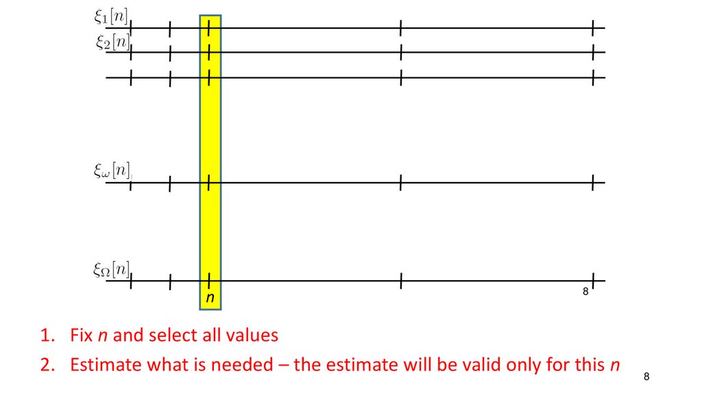
7. Set of realizations

8.

n
8
1. Fix n and select all values
2. Estimate what is needed – the estimate will be valid only for this n
8

9. Range of the random signal

• Discrete range
• Coin flipping
• Dice
• Roulette
• Bits from a communication channel
• Real range
• Strength of wind
• Audio
• CZK/EUR Exchange rate
• etc
9

10. Examples of data I

Discrete data
• 50 years of roulette W = 50 x 365 = 18250 realizations
• Each realization (each playing day) has N=1000 games
(samples)
• Goal: find if someone doesn’t want to cheat the casino
#discrete_data
10

11. Examples of data II

Continuous data
• W = 1068 realizations of flowing water
• Each realization has 20 ms, Fs=16 kHz, so that N=320.
• Goal: find some spectral properties of tubing (eventually to use
running water as a musical instrument)
#continuous_data
11

12. Agenda

13. Describing random signal by functions

• CDF - cummulative distribution function (distribuční funkce)
• x is nothing random ! It is a value, for which we want to
determine/measure CDF. For example, for „which percentage of
population is shorter than 165cm?“, x=165
13

14. Estimation of probabilities of anything

15. Estimation of CDF from data

F(x,n)
x
How to divide x axis ?
• Sufficiently fine
• But not useful in case the estimate is all the time the
same.
15

16.

16
n
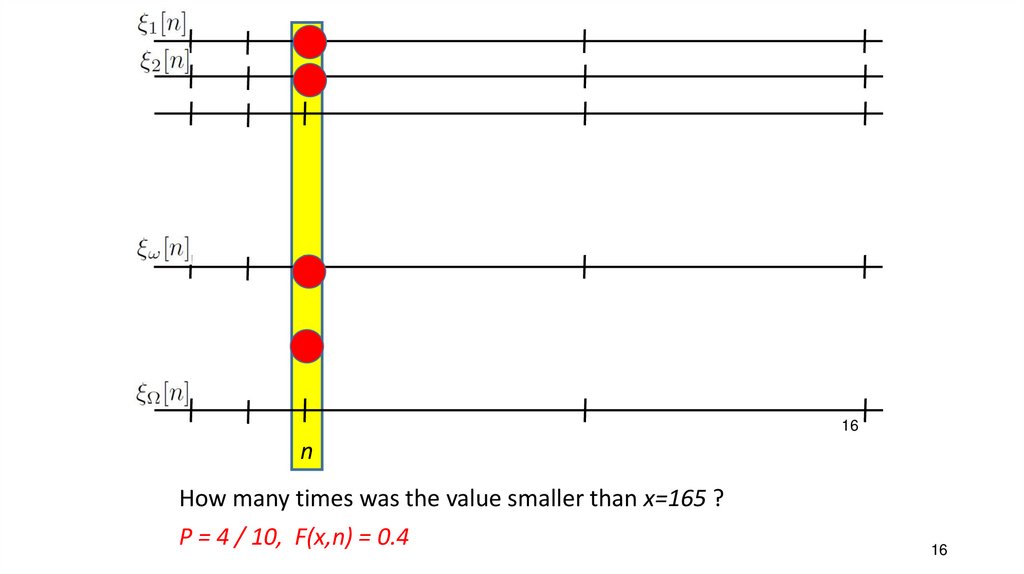
How many times was the value smaller than x=165 ?
P = 4 / 10, F(x,n) = 0.4
16

17. Estimations on our data

• Pick a time n
• Divide the x-axis into reasonable intervals
• Count, over all realizations ω = 1 … W, how many times the value of
signal ξω[n] is smaller than x.
• Divide by the number of realizations
• Plot the results
#cdf_discrete
#cdf_continuous
17

18. Probabilities of values

• Discrete range - OK
• The mass of probabilities is
• Estimation using the counts
18

19.

0
1
2
36
19

20. Estimations on our discrete data

• Pick a time n
• Go over all possible values Xi
• Count, over all realizations ω = 1 … W, how many times the value
of signal ξω[n] is Xi.
• Divide by the number of realizations
• Plot the results
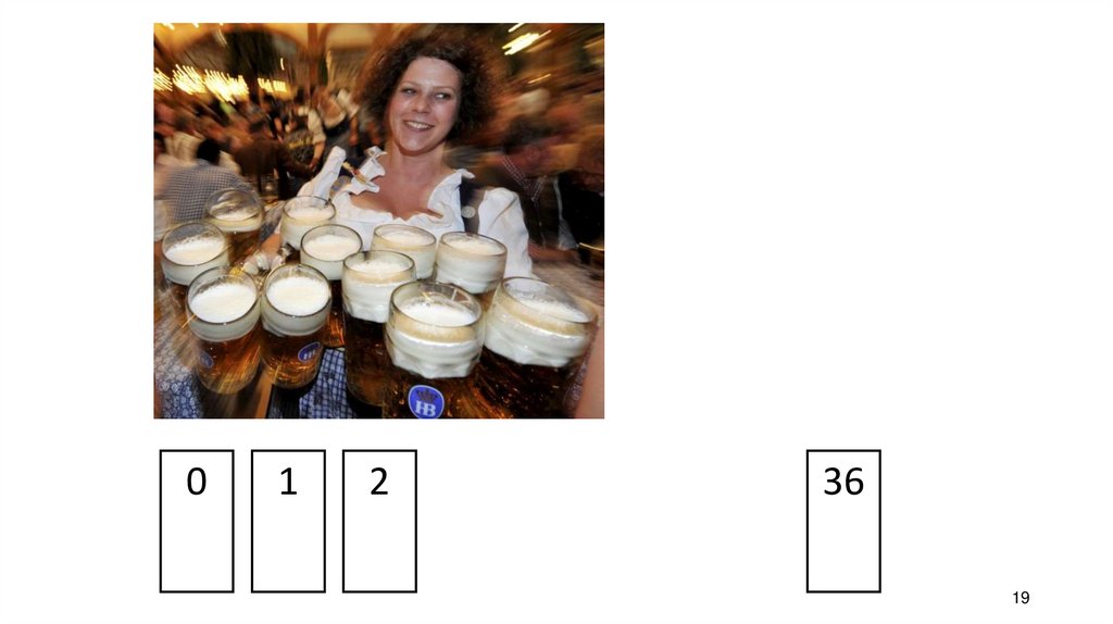
Example for roulette: n = 501, possible values Xi are 0 … 36, in case the
roulette is well balanced, we should see probabilities around 1 / 37 =
0.027
Don’t see the same values ?
#proba_discrete
Not enough data !
20

21. Continuous range

• Nonsense or zero …
=> Needs probability density!
21

22. Real world examples

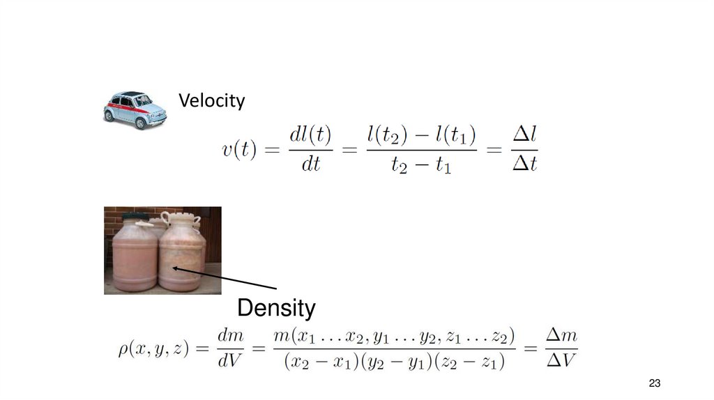
How many kms did the car run at time t ???
What is the mass of the ferment
here, in coordinates x,y,z ???
22

23.

Velocity
Density
23

24. Probability density function – PDF (funkce hustoty rozdělení pravděpodobnosti)

• Is defined as the derivation of cummulative distribution
function over x
• Can be computed numerically
(remember the 1st lecture on the
math).
#pdf_continuous_derivation
• However, we might need
something easier to estimate
PDF directly from the data
24

25. Can we estimate it more easily?

Let us use what we know about the other densities – we need to define
intervals
• Velocity can be estimated as distance driven over an interval of time
(1D interval)
• Physical density can be estimated as a mass over a small volume (3D
interval)
• Probability density can be estimated as probability over an interval
on the axis x
Probabilities of values are
nonsense, but we can use
probabilities of intervals –25bins !

26. Steps of PDF estimation from data

1. Define suitable bins - intervals on the x-axis, uniform intervals with
the width of Δ will make estimation easier.
2. Estimate a histogram – counts of data values in individual bins
3. Convert histogram to probabilities over individual bins – divide by
the number of realizations
4. Convert probabilities to probability densities – divide by width
of bins:
#pdf_continuous_histogram
26

27. Check - the whole thing

How about the integral of density
over all values of the variable ?
• Integral of velocity over the whole
time is the total distance
• Integral of physical density over the
whole volume is the total mass
• Integral of probability density
over all values of variable x is the
total mass of probability = 1
• We can verify this numerically
#total_mass_check
27

28. Agenda

29. Joint probability or joint probability density function

• We want to study relations between samples in different times
• Good for studying dependencies in time
• And later for spectral analysis
• Are they independent or is there a link ?
• We define joint probabilities (sdružené pravděpodobnosti) for signals
with discrete values
• and joint probability density function (sdruženou funkci hustoty
rozdělení pravděpodobnosti) for signals with continuous values
29

30. Principle - counting in two different times

n1
n2
30

31. Estimations – questions, with “and”

Something
at time n1
and
Something
at time n2
31

32. Estimating joint probabilities P(Xi , Xj , ni , nj) for discrete data

• Pick two interesting times: ni and nj
• Go over all possible combinations of values Xi and Xj
• Count, over all realizations ω = 1 … W, how many times the value of
signal ξω[ni] is Xi and the value of signal ξω[nj] is Xj
• Divide by the number of realizations
• Plot the results in some nice 3D plot
Example for roulette: ni = 10, nj = 11, values of Xi are 0 … 36, and values
of Xj as well 0 … 36
#joint_probabilities_discrete
32

33. Interpretting the results

• ni = 10, nj = 11: values of P(Xi, Xj, ni, nj) are noisy but more or less
around 1 / 372 = 0.00073 which is expected for a well balanced
roulette.
Don’t see the same values ?
Not enough data !
• ni = 10, nj = 10: we are looking et the same time, therefore, we will
see probabilities of P(Xi, n) on the diagonal, 1 / 37 = 0.027
• ni = 10, nj = 13: something suspicious ! Why is the value
of P(Xi =3, Xj =32, ni =10, nj =11) much higher than the others ?
• Try also for other pairs of ni and nj with nj - ni = 3 !
33

34. Continuous range – joint probability density function

• As for estimation of probability density function for one
time: p(x,n), probabilities will not work…
• We will need to proceed with a 2D histogram and
perform normalization.
• Remember, we ask again a question about two times
and two events.
Something
at time n1
and
Something
at time n2
34

35. Estimation of joint PDF in bins

1. An interval at time n1 on axis x1, and an interval at time n2 on axis
x2, define a 2-dimensional (square) bin. Uniform intervals with the
width of Δ will make estimation easier.
2. Estimate a histogram – counts of data values in individual bins
3. Convert histogram to probabilities over individual bins – divide by
the number of realizations
4. Convert probabilities to probability densities – divide by surface
of bins:
#joint_pdf_histogram
35

36. Example of joint PDF estimation for water

• times n1 = 10, n2 = 11
• Dividing both x1 and x2 with
the step of Δ = 0.03
• The 2D bins are therefore
squares Δ x Δ, with
surface of 0.0009
Interpretation of joint PDF: in
case the value at n1 is
positive, it is likely that value
at n2 is also positive –
correlation.
2D bin
36

37. Joint PDF - n1 = 10, and n2 = 10

• the same sample, the values of p(x1, x2, n1, n2) are on the diagonal
and correspond to the standard (not joint) PDF p(x, n)
37

38. Joint PDF - n1 = 10, and n2 = 16

• Can not say much about sample at time n2 knowing the sample at
time n1 – no correlation.
38

39. Joint PDF - n1 = 10, and n2 = 23

• in case the value at n1 is positive, it is likely that value at n2 is negative
– negative correlation, anti-correlation.
39

40. Agenda

41. Moments (momenty)

• Single numbers characterizing the random signal.
• We are still fixed at time n !
• A moment is an Expectation (očekávaná hodnota) of something
Expectation = sum all possible values of x
probability of x
times the thing that we’re expecting
The computation depends on the character of the random signal
• Sum for discrete values (we have probabilities)
• Integral for continuous values (we have probability densities).
41

42. Mean value (střední hodnota)

• Expectation of the value
• “what we’re expecting” is just the value.
• Discrete case – discrete values Xi, probabilities P(Xi, n), we sum.
#mean_discrete
• Continuous case – continuous variable x, probability density p(x,n), we
integrate.
#mean_continuous
In the demos, pay attention to visualization of the
product “probability (or density) times the thing that we’re expecting” !
42

43. Variance (dispersion, variance, rozptyl)

• Expectation of the zero-mean and squared value
• Related to energy, power …
• Discrete case – discrete values (Xi - a[n])2, probabilities P(Xi , n), we sum.
#variance_discrete
• Continuous case – continuous values (x - a[n])2, probability density p(x,n),
we integrate.
#variance_continuous
In the demos, pay again attention to visualization of the
product “probability (or density) times the thing that we’re expecting” !
43

44. Ensemble estimates of mean and variance

45. Just select data and use formulas known from high school !

• Discrete values
#mean_variance_estimation_discrete
• Continuous values
#mean_variance_estimation_continuous
Cool, the formulas are exactly the same !
45

46. Agenda

47. Correlation coefficient (korelační koeficient)

• Expectation of the product of values at two different times
• One value characterizing the relation
of two different times
• Discrete case – discrete values Xi and Xj, joint probabilities P(Xi , Xj , ni , nj),
we double-sum (over all values of Xi and over all values of Xj ).
#corrcoef_discrete
• Continuous case – continuous values xi and xj, joint probability density
function p(xi , xj , ni , nj), we double-integrate (over all values of xi and over
all values of xj).
#corrcoef_continuous
In the demos, pay again attention
to visualization of the product “probability (or density) times the thing that
we’re expecting” (this time in 2D) !
47

48. Discrete case

• n1 = 10, n2 = 11
• Some correlation
• But the values have mean
value … if we remove it
• 323.6 – 182 = -0.4, this is
almost zero …
No correlation
48 / 72

49. Discrete case

• n1 = 10, n2 = 10
• The same time
Maximum correlation
49 / 72

50. Discrete case

• n1 = 20, n2 = 23
• value … if we remove it
• 326.2 – 182 = 2.2,
• This can mean something !
50 / 72

51. Continuous case

• n1 = 10, n2 = 11
• Try to imagine the product
xi xj – saddle function
(sedlová funkce)
• The colormaps were
modified to show positive
values in red and negative
in blue
• Positive parts prevalent
Correlated
51 / 72

52. Continuous case

• n1 = 10, n2 = 10
• The same time
Maximum correlation
52 / 72

53. Continuous case

• n1 = 10, n2 = 16
• Can’t say anything about
sample at time n2 knowing
the sample at time n1
• Positive parts cancel
the negative ones
No correlation
53 / 72

54. Continuous case

• n1 = 10, n2 = 23
• If sample at time n1 is
positive, sample at time n2
will be probably negative
and vice versa
• Negative parts prevalent
Negative correlation,
anti-correlation
54 / 72

55. Direct ensemble estimate of correlation coefficient

n1
n2

56. Just select data and multiply the two samples in each realization + normalize

• Discrete values
#corrcoef_estimation_discrete
• Continuous values
#corrcoef_estimation_continuous
Cool, the formulas are again exactly the same !
56

57.

Computing a sequence of correlation coefficients: n1 fixed and n2
varying from n1 to some value …
• Discrete values – not sure if very useful …
#corrcoef_sequence_discrete
• Continuous values – can bring interesting information about the
spectrum.
#corrcoef_sequence_continuous
57

58. Agenda

59. Stationarity (stacionarita)

• The behavior of stationary random signal does not change over time
(or at least we believe that it does not…)
• Values and functions independent on time n
• Correlation coefficients do not depend on n1 and n2, only on their
difference k=n2-n1
59

60. Checking the stationarity

• Are cumulative distribution functions F(x,n) approximately the same
for all samples n? (visualize a few)
• Are probabilities approximately the same for all samples n? (visualize
a few)
• Discrete: probabilities P(Xi , n)
• Continuous: probability density functions p(x, n)
• Are means a[n] approximately the same for all samples n ?
• Are variances D[n] approximately the same for all samples n ?
• Are correlation coefficients depending only on the distance k = n2 – n1
and not on the absolute position ?
60

61. Results

#stationarity_check_discrete
#stationarity_check_continuous
61

62. Agenda

63. Ergodicity

• The parameters can be estimated from one single realization –
temporal estimates (časové odhady)
… or at least we hope
… most of the time, we’ll have to do it anyway, so at least trying to
make it as long as we can.
… however, we should have stationarity in mind – compromises must
be done for varying signals (speech, music, video …)
63

64. Temporal estimates

• All estimations will be running on one realization
• All sums going over realizations will be replaced by sums running over
time.
#ergodic_discrete
#ergodic_continuous
64

65. We can even do temporal estimates of joint probabilities !

• As above, replacing counting over realizations by counting over time.
#ergodic_joint_probabilities
For k = 0, 1, 2, 3
65

66. Agenda

67. SUMMARY

• Random signals are of high interest
• Everywhere around us
• They carry information
• Discrete vs. continuous range
• Can not precisely define them, other means of description
• Set of realizations
• Functions – cumulative distribution, probabilities, probability density
• Scalars – moments
• Behavior between two times
• Functions: joint probabilities or joint PDFs.
• Scalars: correlation coefficients
67

68. SUMMARY II.

• Counts
• of an event „how many times did you see the water signal in interval 5 to 10?“
• Probabilities
• Estimated as count / total.
• Probability density
• Estimated as Probability / size of interval (1D or 2D)
• In case we have a set of realizations – ensemble estimates.
68

69. SUMMARY III.

• Stationarity – behavior not depending on time.
• Ergodicity – everything can be estimated from one realization
• Temporal estimates
69

70. TODO’s

• More on correlation coefficients and their estimation
• Spectral analysis of random signals and their filtering
• What is white noise and why is it white.
• How does quantization work and how can random signals help us in
determining the SNR (signal to noise ratio) caused by quantization.
70

English Русский Правила