Random signals II

1. Random signals II

Honza Černocký, ÚPGM
Please open Python notebook random_2

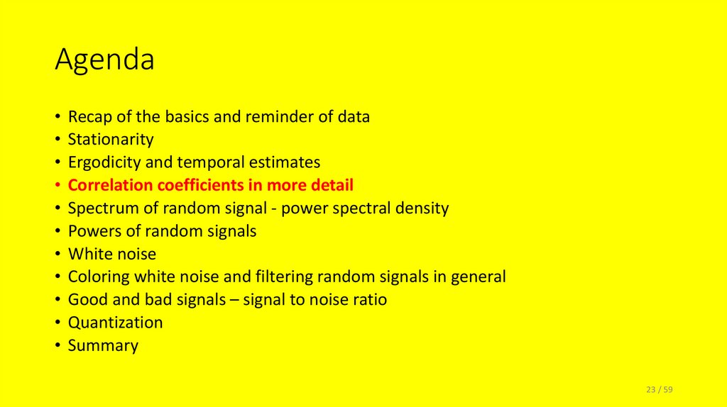
2. Agenda

• Recap of the basics and reminder of data
• Stationarity
• Ergodicity and temporal estimates
• Correlation coefficients in more detail
• Spectrum of random signal - power spectral density
• Powers of random signals
• White noise
• Coloring white noise and filtering random signals in general
• Good and bad signals – signal to noise ratio
• Quantization
• Summary
2 / 59

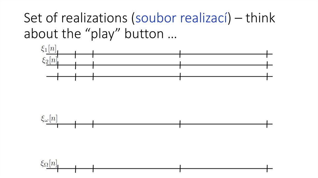
3. Set of realizations (soubor realizací) – think about the “play” button …

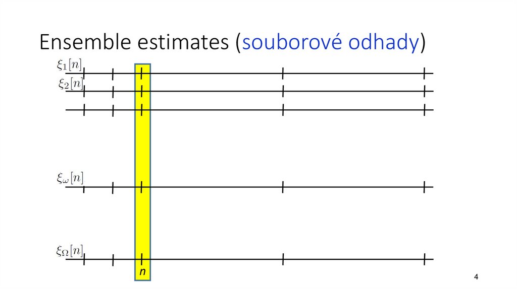
4. Ensemble estimates (souborové odhady)

n
4

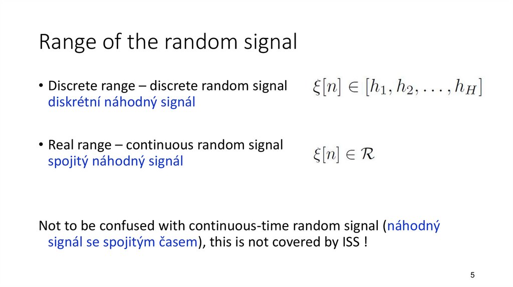
5. Range of the random signal

• Discrete range – discrete random signal
diskrétní náhodný signál
• Real range – continuous random signal
spojitý náhodný signál
Not to be confused with continuous-time random signal (náhodný
signál se spojitým časem), this is not covered by ISS !
5

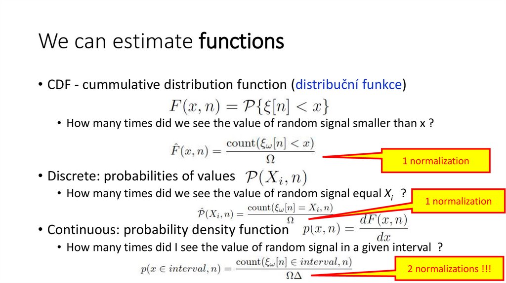
6. We can estimate functions

• CDF - cummulative distribution function (distribuční funkce)
• How many times did we see the value of random signal smaller than x ?
1 normalization
• Discrete: probabilities of values
• How many times did we see the value of random signal equal Xi ?
1 normalization
• Continuous: probability density function
• How many times did I see the value of random signal in a given interval ?
2 normalizations
!!!
6

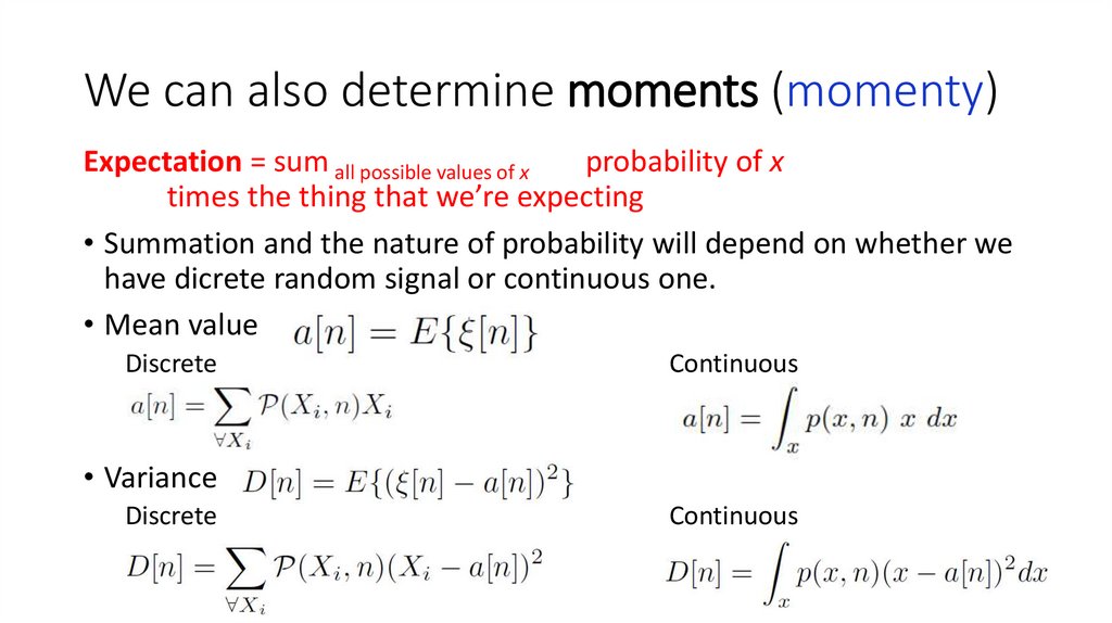
7. We can also determine moments (momenty)

Expectation = sum all possible values of x
probability of x
times the thing that we’re expecting
• Summation and the nature of probability will depend on whether we
have dicrete random signal or continuous one.
• Mean value
Discrete
Continuous
• Variance
Discrete
Continuous
7

8. We can estimate moments directly from the ensemble of realizations

• Ouff1: we know these from high school …
• Ouff2: we don’t have to care whether the signal has discrete or
continuous values
8

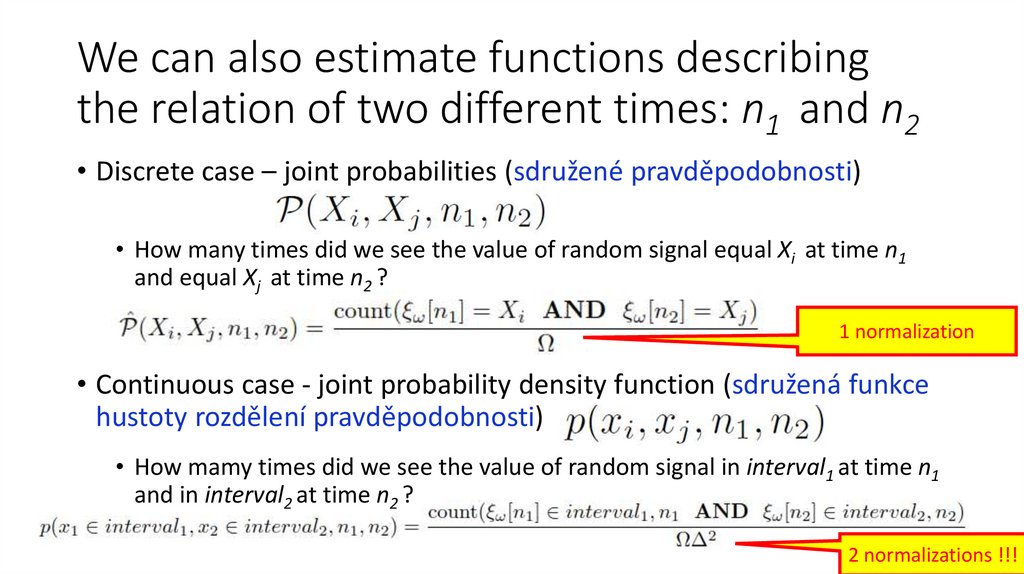
9. We can also estimate functions describing the relation of two different times: n1 and n2

• Discrete case – joint probabilities (sdružené pravděpodobnosti)
• How many times did we see the value of random signal equal Xi at time n1
and equal Xj at time n2 ?
1 normalization
• Continuous case - joint probability density function (sdružená funkce
hustoty rozdělení pravděpodobnosti)
• How mamy times did we see the value of random signal in interval1 at time n1
and in interval2 at time n2 ?
9
2 normalizations
!!!

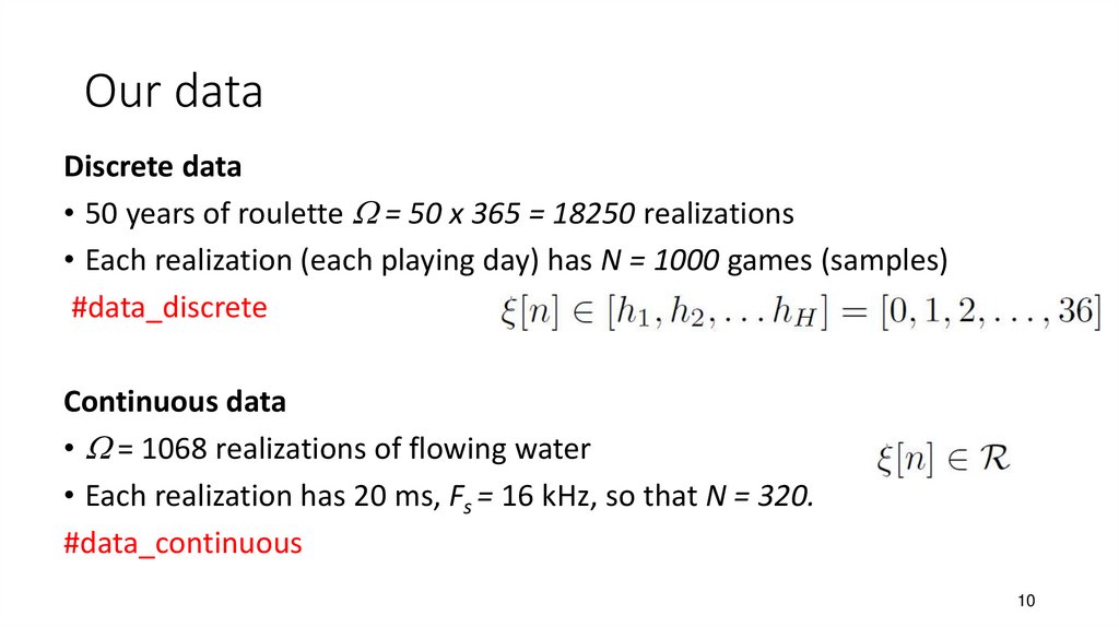
10. Our data

Discrete data
• 50 years of roulette W = 50 x 365 = 18250 realizations
• Each realization (each playing day) has N = 1000 games (samples)
#data_discrete
Continuous data
• W = 1068 realizations of flowing water
• Each realization has 20 ms, Fs = 16 kHz, so that N = 320.
#data_continuous
10

11. Agenda

• Recap of the basics and reminder of data
• Stationarity
• Ergodicity and temporal estimates
• Correlation coefficients in more detail
• Spectrum of random signal - power spectral density
• Powers of random signals
• White noise
• Coloring white noise and filtering random signals in general
• Good and bad signals – signal to noise ratio
• Quantization
• Summary
11 / 59

12. Does the random signal behave the same way over the time ?

• So far, we did ensemble estimates for each time n or each pair of
times n1, n2 independently.
• This takes lots of time, and we would like to have one function or one
value to describe the whole random signal.
Remember: the signal can NOT have the same or deterministic
samples, it is random !
12 / 59

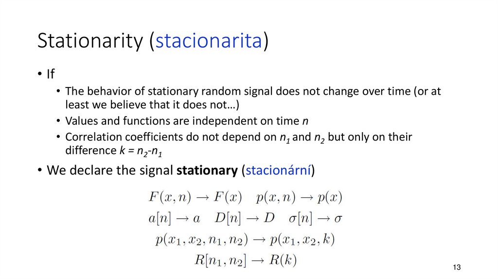
13. Stationarity (stacionarita)

• If
• The behavior of stationary random signal does not change over time (or at
least we believe that it does not…)
• Values and functions are independent on time n
• Correlation coefficients do not depend on n1 and n2 but only on their
difference k = n2-n1
• We declare the signal stationary (stacionární)
13

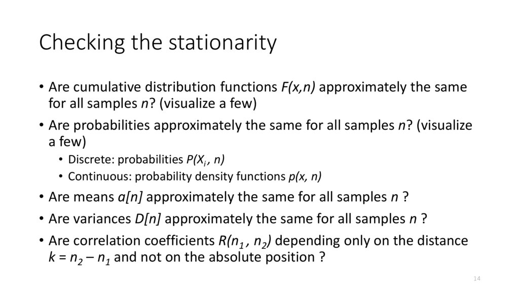
14. Checking the stationarity

• Are cumulative distribution functions F(x,n) approximately the same
for all samples n? (visualize a few)
• Are probabilities approximately the same for all samples n? (visualize
a few)
• Discrete: probabilities P(Xi , n)
• Continuous: probability density functions p(x, n)
• Are means a[n] approximately the same for all samples n ?
• Are variances D[n] approximately the same for all samples n ?
• Are correlation coefficients R(n1 , n2) depending only on the distance
k = n2 – n1 and not on the absolute position ?
14

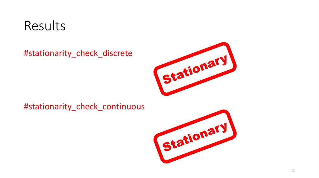
15. Results

#stationarity_check_discrete
#stationarity_check_continuous
15

16. Agenda

• Recap of the basics and reminder of data
• Stationarity
• Ergodicity and temporal estimates
• Correlation coefficients in more detail
• Spectrum of random signal - power spectral density
• Powers of random signals
• White noise
• Coloring white noise and filtering random signals in general
• Good and bad signals – signal to noise ratio
• Quantization
• Summary
16 / 59

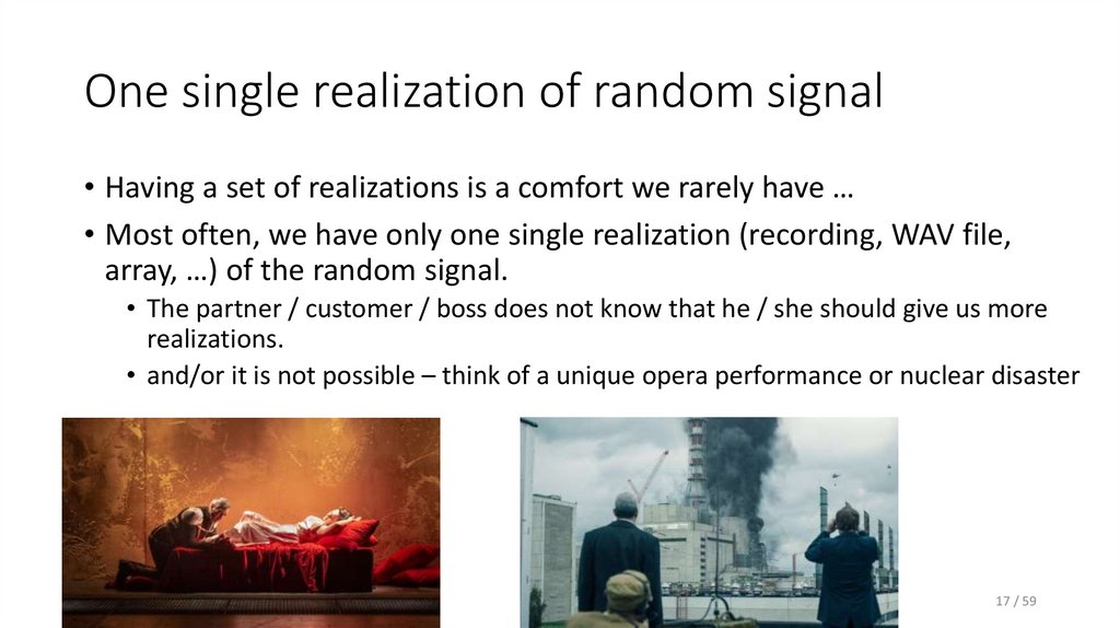
17. One single realization of random signal

• Having a set of realizations is a comfort we rarely have …
• Most often, we have only one single realization (recording, WAV file,
array, …) of the random signal.
• The partner / customer / boss does not know that he / she should give us more
realizations.
• and/or it is not possible – think of a unique opera performance or nuclear disaster
17 / 59

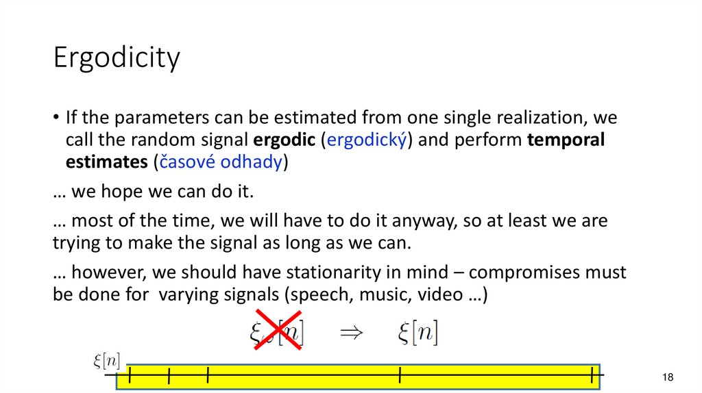
18. Ergodicity

• If the parameters can be estimated from one single realization, we
call the random signal ergodic (ergodický) and perform temporal
estimates (časové odhady)
… we hope we can do it.
… most of the time, we will have to do it anyway, so at least we are
trying to make the signal as long as we can.
… however, we should have stationarity in mind – compromises must
be done for varying signals (speech, music, video …)
18

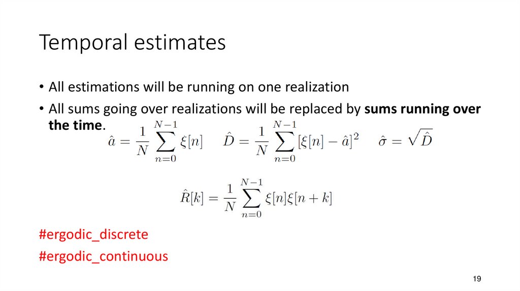
19. Temporal estimates

• All estimations will be running on one realization
• All sums going over realizations will be replaced by sums running over
the time.
#ergodic_discrete
#ergodic_continuous
19

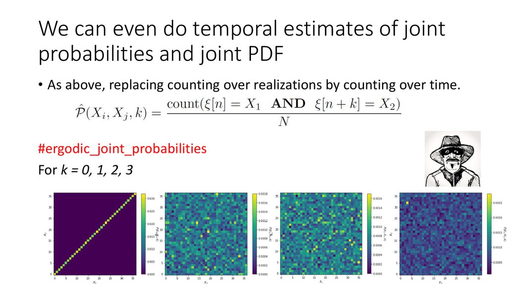
20. We can even do temporal estimates of joint probabilities and joint PDF

• As above, replacing counting over realizations by counting over time.
#ergodic_joint_probabilities
For k = 0, 1, 2, 3
20

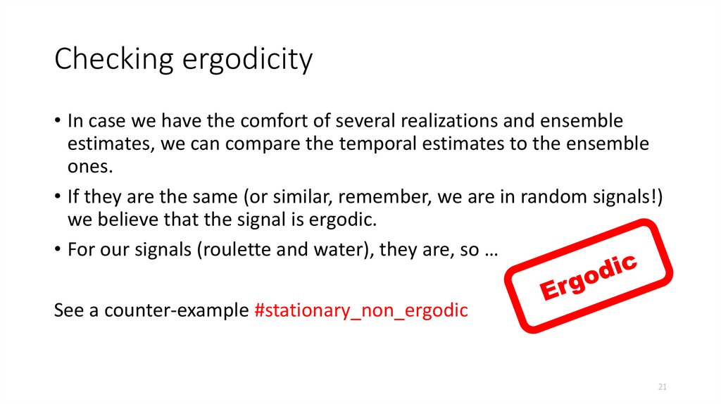
21. Checking ergodicity

• In case we have the comfort of several realizations and ensemble
estimates, we can compare the temporal estimates to the ensemble
ones.
• If they are the same (or similar, remember, we are in random signals!)
we believe that the signal is ergodic.
• For our signals (roulette and water), they are, so …
See a counter-example #stationary_non_ergodic
21

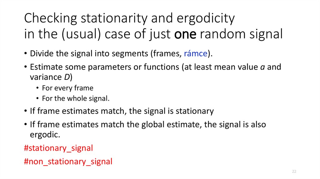
22. Checking stationarity and ergodicity in the (usual) case of just one random signal

• Divide the signal into segments (frames, rámce).
• Estimate some parameters or functions (at least mean value a and
variance D)
• For every frame
• For the whole signal.
• If frame estimates match, the signal is stationary
• If frame estimates match the global estimate, the signal is also
ergodic.
#stationary_signal
#non_stationary_signal
22

23. Agenda

• Recap of the basics and reminder of data
• Stationarity
• Ergodicity and temporal estimates
• Correlation coefficients in more detail
• Spectrum of random signal - power spectral density
• Powers of random signals
• White noise
• Coloring white noise and filtering random signals in general
• Good and bad signals – signal to noise ratio
• Quantization
• Summary
23 / 59

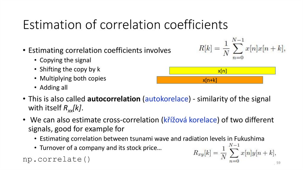
24. Estimation of correlation coefficients

• Estimating correlation coefficients involves
• Copying the signal
• Shifting the copy by k
• Multiplying both copies
• Adding all
x[n]
x[n+k]
• This is also called autocorrelation (autokorelace) - similarity of the signal
with itself Rxx[k].
• We can also estimate cross-correlation (křížová korelace) of two different
signals, good for example for
• Estimating correlation between tsunami wave and radiation levels in Fukushima
• Turnover of a company and its stock price…
np.correlate()
24 / 59

25. Biased estimate (vychýlený odhad) of R[k]

• Signal has samples 0 … N-1, we can run k from –(N-1) to N-1
• We divide by the same number of samples N,
• k = 0: highest number of samples (N) for the estimation
x[n]
=> high value
x[n+k]
• Small k: still plenty of samples for the estimation
=> still high value
x[n]
x[n+k]
• Big k: few samples for the estimation
=> low value
x[n]
x[n+k]
#biased_Rk_estimate
25 / 59

26. Unbiased estimate (nevychýlený odhad) of R[k]

• Dividing always by N penalizes the values of R[k] for higher values of k.
• Change the definition of R[k] so that we always divide
only by the number of “active” samples.
• N-k works for positive k’s
• k can also be negative, so N-|k| is more general
• Unbiased estimate of correlation coefficients
Justice for
correlation
coefficients !
26 / 59

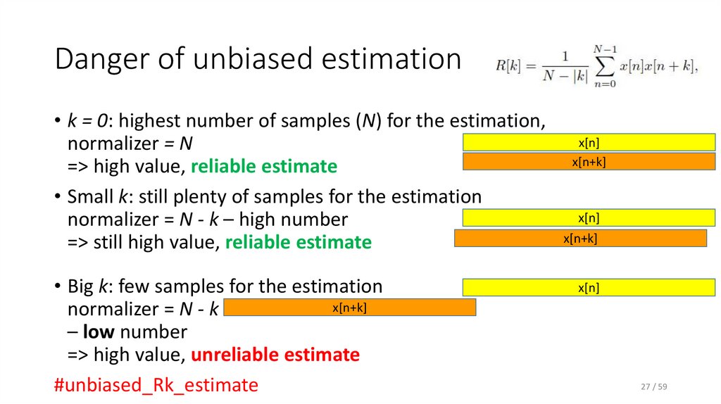
27. Danger of unbiased estimation

• k = 0: highest number of samples (N) for the estimation,
normalizer = N
=> high value, reliable estimate
• Small k: still plenty of samples for the estimation
normalizer = N - k – high number
=> still high value, reliable estimate
• Big k: few samples for the estimation
x[n+k]
normalizer = N - k
– low number
=> high value, unreliable estimate
#unbiased_Rk_estimate
x[n]
x[n+k]
x[n]
x[n+k]
x[n]
27 / 59

28. Agenda

• Recap of the basics and reminder of data
• Stationarity
• Ergodicity and temporal estimates
• Correlation coefficients in more detail
• Spectrum of random signal - power spectral density
• Powers of random signals
• White noise
• Coloring white noise and filtering random signals in general
• Good and bad signals – signal to noise ratio
• Quantization
• Summary
28 / 59

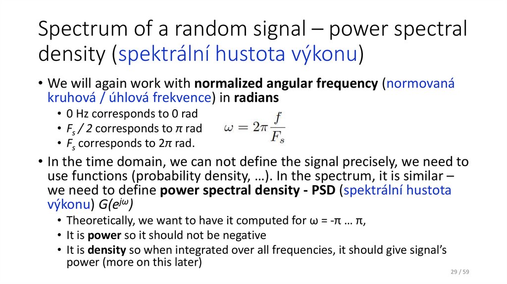
29. Spectrum of a random signal – power spectral density (spektrální hustota výkonu)

• We will again work with normalized angular frequency (normovaná
kruhová / úhlová frekvence) in radians
• 0 Hz corresponds to 0 rad
• Fs / 2 corresponds to π rad
• Fs corresponds to 2π rad.
• In the time domain, we can not define the signal precisely, we need to
use functions (probability density, …). In the spectrum, it is similar –
we need to define power spectral density - PSD (spektrální hustota
výkonu) G(ejω)
• Theoretically, we want to have it computed for ω = -π … π,
• It is power so it should not be negative
• It is density so when integrated over all frequencies, it should give signal’s
power (more on this later)
29 / 59

30. Estimating G(ejω)

jω
Estimating G(e )
• Remember that in classical spectrum computation, we used Discrete
time Fourier transform – DTFT (Fourierova transformace s diskrétním
časem)
• For random signals, we need a reliable representation of the signal in
time – we use correlation coefficients R[k].
• Conversion of R[k] to G(ejω) is given
by Wiener-Khinchin (Хинчин) theorem:
• PSD is symmetrical for positive and negative frequency:
30 / 59

31. Practical hints for estimating G(ejω) from R[k]

jω
Practical hints for estimating G(e ) from R[k]
• DTFT - will be of course computed by DFT/FFT.
• Number of correlation coefficients is usually not a power of 2 – good to limit it to
power of two.
• DFT does not accept negative coefficients, but we can flip R[-k] to R[N-k] by
np.fft.fftshift
• As the input is symmetrical, the result should be real, but we better force it to be
real by np.real
• When DFT is computed, it gives us output for ω = 0 … 2π, we can use
np.fft.fftshift, if we want the symmetric picture.
• As correlation coefficients for higher k’s can be noisy, we can set them to zero attention, if zeroing R[k], we need to zero also R[N-k] to preserve the symmetry.
• Your boss / customer / partner will probably ask just for frequencies
from 0 to Fs /2 and in Hz
#power_spec_density_from_Rk
31 / 59

32. Estimating PSD directly from the signal

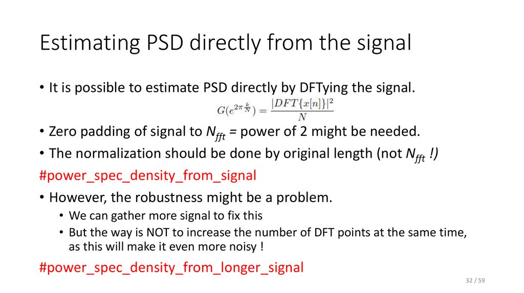
• It is possible to estimate PSD directly by DFTying the signal.
• Zero padding of signal to Nfft = power of 2 might be needed.
• The normalization should be done by original length (not Nfft !)
#power_spec_density_from_signal
• However, the robustness might be a problem.
• We can gather more signal to fix this
• But the way is NOT to increase the number of DFT points at the same time,
as this will make it even more noisy !
#power_spec_density_from_longer_signal
32 / 59

33. Making DFT estimation of PSD more robust

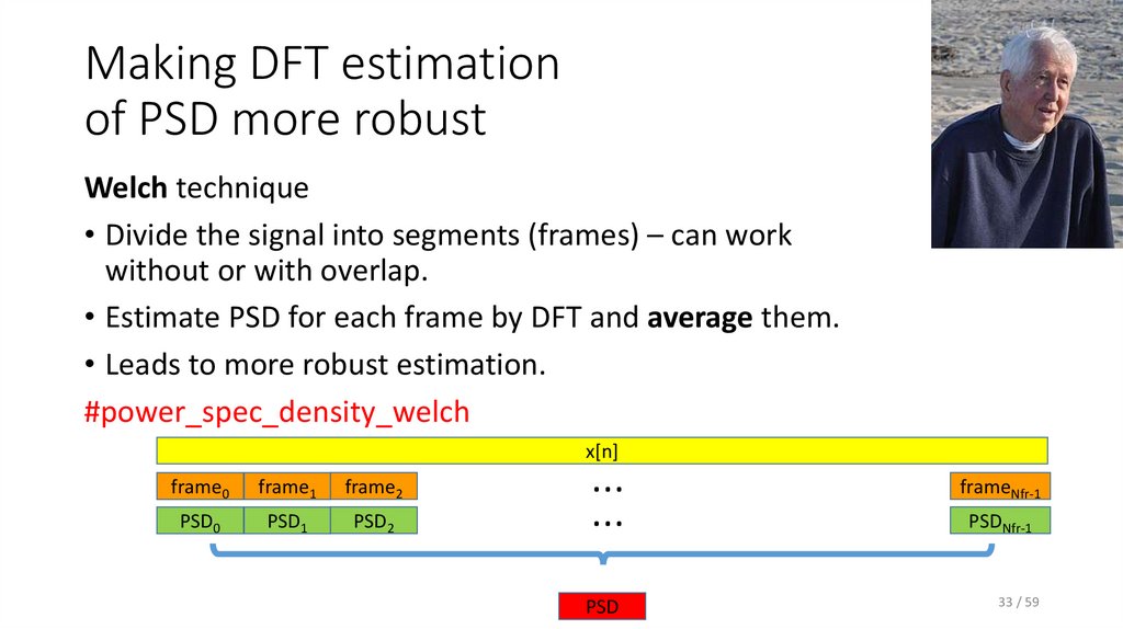
Welch technique
• Divide the signal into segments (frames) – can work
without or with overlap.
• Estimate PSD for each frame by DFT and average them.
• Leads to more robust estimation.
#power_spec_density_welch
x[n]
frame0
frame1
frame2
PSD0
PSD1
PSD2
…
…
frameNfr-1
PSD
33 / 59
PSDNfr-1

34. Agenda

• Recap of the basics and reminder of data
• Stationarity
• Ergodicity and temporal estimates
• Correlation coefficients in more detail
• Spectrum of random signal - power spectral density
• Powers of random signals
• White noise
• Coloring white noise and filtering random signals in general
• Good and bad signals – signal to noise ratio
• Quantization
• Summary
34 / 59

35. Several ways to compute power of random signal

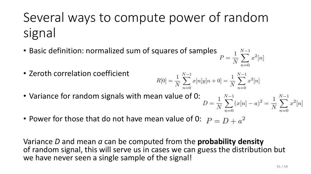
• Basic definition: normalized sum of squares of samples
• Zeroth correlation coefficient
• Variance for random signals with mean value of 0:
• Power for those that do not have mean value of 0:
Variance D and mean a can be computed from the probability density
of random signal, this will serve us in cases we can guess the distribution but
we have never seen a single sample of the signal!
35 / 59

36. Several ways to compute power of random signal II

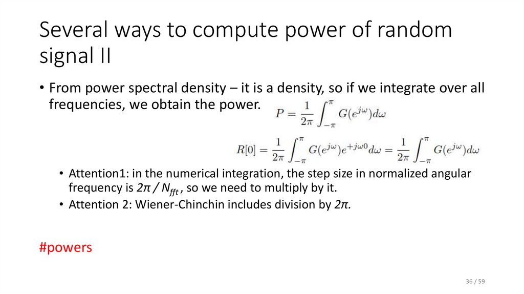
• From power spectral density – it is a density, so if we integrate over all
frequencies, we obtain the power.
• Attention1: in the numerical integration, the step size in normalized angular
frequency is 2π / Nfft , so we need to multiply by it.
• Attention 2: Wiener-Chinchin includes division by 2π.
#powers
36 / 59

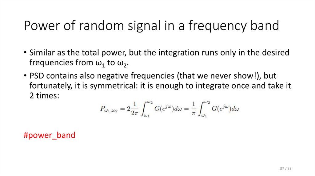
37. Power of random signal in a frequency band

• Similar as the total power, but the integration runs only in the desired
frequencies from ω1 to ω2.
• PSD contains also negative frequencies (that we never show!), but
fortunately, it is symmetrical: it is enough to integrate once and take it
2 times:
#power_band
37 / 59

38. Agenda

• Recap of the basics and reminder of data
• Stationarity
• Ergodicity and temporal estimates
• Correlation coefficients in more detail
• Spectrum of random signal - power spectral density
• Powers of random signals
• White noise
• Coloring white noise and filtering random signals in general
• Good and bad signals – signal to noise ratio
• Quantization
• Summary
38 / 59

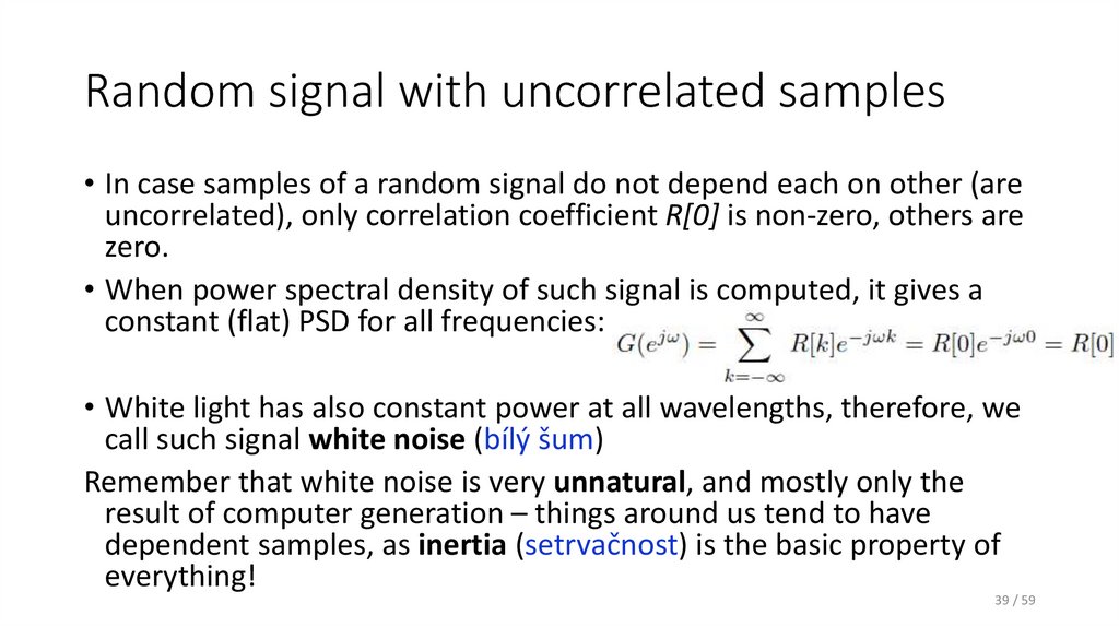
39. Random signal with uncorrelated samples

• In case samples of a random signal do not depend each on other (are
uncorrelated), only correlation coefficient R[0] is non-zero, others are
zero.
• When power spectral density of such signal is computed, it gives a
constant (flat) PSD for all frequencies:
• White light has also constant power at all wavelengths, therefore, we
call such signal white noise (bílý šum)
Remember that white noise is very unnatural, and mostly only the
result of computer generation – things around us tend to have
dependent samples, as inertia (setrvačnost) is the basic property of
everything!
39 / 59

40. Uniform white noise

• The values of samples follow uniform distribution, from some –Δ/2 to
Δ/2.
#uniform_white_noise
40 / 59

41. Gaussian white noise

• The values of samples follow standard normal (Gaussian) distribution,
with mean μ and standard deviation σ.
#gaussian_white_noise
41 / 59

42. White noise with discrete values

• Even binary noise producing values -1 and +1 can be white !
• Probabilities P(-1) = 0.5, P(+1) = 0.5.
#binary_white_noise
Whiteness does not depend on the distribution of the samples, it is
given by the independence (non-correlation) of samples !
42 / 59

43. White noise PSD estimation by DFT from signal

• By taking one DFT, the estimate is so unreliable, that we are not able
recognize the theoretical (flat) PSD !
• Using Welch method is obligatory
• Split in frames
• Compute PSD for each
• Average
#white_noise_psd_by_dft
43 / 59

44. Agenda

• Recap of the basics and reminder of data
• Stationarity
• Ergodicity and temporal estimates
• Correlation coefficients in more detail
• Spectrum of random signal - power spectral density
• Powers of random signals
• White noise
• Coloring white noise and filtering random signals in general
• Good and bad signals – signal to noise ratio
• Quantization
• Summary
44 / 59

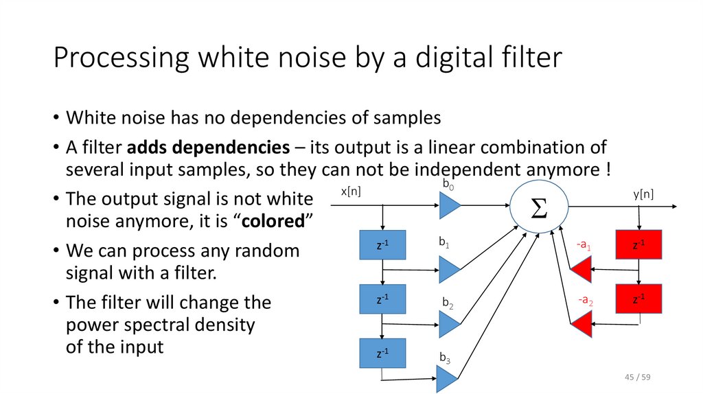
45. Processing white noise by a digital filter

• White noise has no dependencies of samples
• A filter adds dependencies – its output is a linear combination of
several input samples, so they can not be independent anymore !
b0
x[n]
• The output signal is not white
S
noise anymore, it is “colored”
b1
-a1
z-1
• We can process any random
signal with a filter.
-a2
z-1
b2
• The filter will change the
power spectral density
of the input
z-1
b
y[n]
z-1
z-1
3
45 / 59

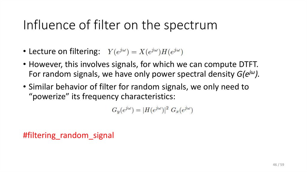
46. Influence of filter on the spectrum

• Lecture on filtering:
• However, this involves signals, for which we can compute DTFT.
For random signals, we have only power spectral density G(ejω).
• Similar behavior of filter for random signals, we only need to
“powerize” its frequency characteristics:
#filtering_random_signal
46 / 59

47. Agenda

• Recap of the basics and reminder of data
• Stationarity
• Ergodicity and temporal estimates
• Correlation coefficients in more detail
• Spectrum of random signal - power spectral density
• Powers of random signals
• White noise
• Coloring white noise and filtering random signals in general
• Good and bad signals – signal to noise ratio
• Quantization
• Summary
47 / 59

48. Signal to noise ratio

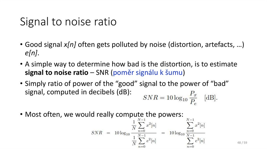
• Good signal x[n] often gets polluted by noise (distortion, artefacts, …)
e[n].
• A simple way to determine how bad is the distortion, is to estimate
signal to noise ratio – SNR (poměr signálu k šumu)
• Simply ratio of power of the “good” signal to the power of “bad”
signal, computed in decibels (dB):
• Most often, we would really compute the powers:
48 / 59

49. SNR practical know-how

• The signal is stronger than noise: Ps > Pe , fraction Ps /Pe > 1, log is > 0
=> Positive SNR.
10dB is 10x bigger power, 20dB is 100x bigger power, etc.
• The signal is weaker than noise: Ps < Pe , fraction Ps /Pe < 1, log is < 0
=> Negative SNR.
-10dB is 10x weaker power, -20dB is 100x weaker power, etc.
• The signal has the same power as noise: Ps = Pe , fraction Ps /Pe = 1,
log 1 = 0 => SNR = 0 dB
• SNR is not almighty (not perceptually based, requires alignment of signals,
etc), but simple to compute and widely used.
• SNR can be easily inverted and we can noise a signal at a specific SNR.
#SNR_examples
49 / 59

50. Agenda

• Recap of the basics and reminder of data
• Stationarity
• Ergodicity and temporal estimates
• Correlation coefficients in more detail
• Spectrum of random signal - power spectral density
• Powers of random signals
• White noise
• Coloring white noise and filtering random signals in general
• Good and bad signals – signal to noise ratio
• Quantization
• Summary
50 / 59

51. Principles of quantization (kvantování)

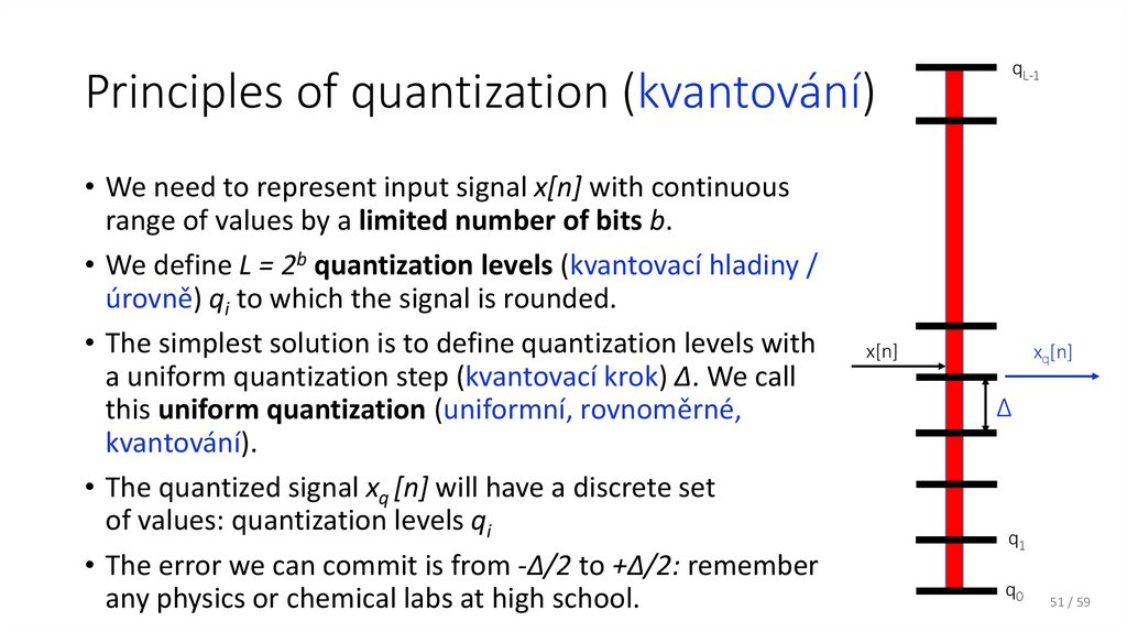
• We need to represent input signal x[n] with continuous
range of values by a limited number of bits b.
• We define L = 2b quantization levels (kvantovací hladiny /
úrovně) qi to which the signal is rounded.
• The simplest solution is to define quantization levels with
a uniform quantization step (kvantovací krok) Δ. We call
this uniform quantization (uniformní, rovnoměrné,
kvantování).
• The quantized signal xq [n] will have a discrete set
of values: quantization levels qi
• The error we can commit is from -Δ/2 to +Δ/2: remember
any physics or chemical labs at high school.
qL-1
x[n]
xq[n]
Δ
q1
q0
51 / 59

52. How much do we harm the signal by quantization ?

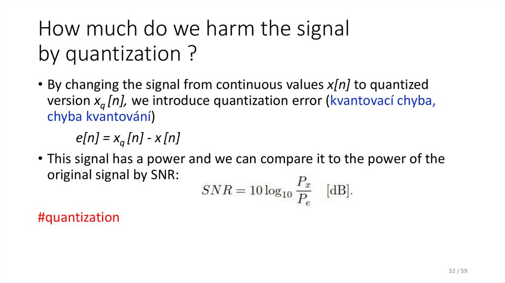
• By changing the signal from continuous values x[n] to quantized
version xq [n], we introduce quantization error (kvantovací chyba,
chyba kvantování)
e[n] = xq [n] - x [n]
• This signal has a power and we can compare it to the power of the
original signal by SNR:
#quantization
52 / 59

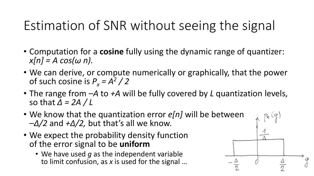
53. Estimation of SNR without seeing the signal

• Computation for a cosine fully using the dynamic range of quantizer:
x[n] = A cos(ω n).
• We can derive, or compute numerically or graphically, that the power
of such cosine is Px = A2 / 2
• The range from –A to +A will be fully covered by L quantization levels,
so that Δ = 2A / L
• We know that the quantization error e[n] will be between
–Δ/2 and +Δ/2, but that’s all we know.
• We expect the probability density function
of the error signal to be uniform
• We have used g as the independent variable
to limit confusion, as x is used for the signal …

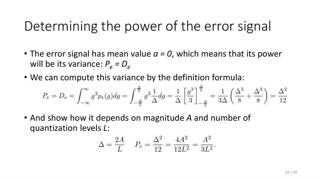
54. Determining the power of the error signal

• The error signal has mean value a = 0, which means that its power
will be its variance: Pe = De
• We can compute this variance by the definition formula:
• And show how it depends on magnitude A and number of
quantization levels L:
54 / 59

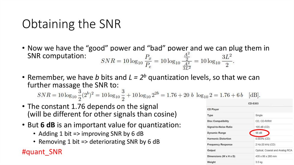
55. Obtaining the SNR

• Now we have the “good” power and “bad” power and we can plug them in
SNR computation:
• Remember, we have b bits and L = 2b quantization levels, so that we can
further massage the SNR to:
• The constant 1.76 depends on the signal
(will be different for other signals than cosine)
• But 6 dB is an important value for quantization:
• Adding 1 bit => improving SNR by 6 dB
• Removing 1 bit => deteriorating SNR by 6 dB
#quant_SNR
55 / 59

56. Agenda

• Recap of the basics and reminder of data
• Stationarity
• Ergodicity and temporal estimates
• Correlation coefficients in more detail
• Spectrum of random signal - power spectral density
• Powers of random signals
• White noise
• Coloring white noise and filtering random signals in general
• Good and bad signals – signal to noise ratio
• Quantization
• Summary
56 / 59

57. Summary I

• Stationarity – behavior of random signal is not depending on time.
• Ergodicity – everything can be estimated from one realization
• Ensemble estimates are replaced by temporal ones.
• Correlation coefficients R[k] can be easily estimated from the signal
• Biased – they will fade for high values of k
• Unbiased – mathematically correct but very unrealiable for high values of k.
• Spectrum of random signals is given by power spectral density (PSD)
• Can be estimated from correlation coefficients by DTFT (Wiener-Khinchin)
• … or directly from the signal, robustness can be an issue, so think about
averaging several estimates (Welch).
57

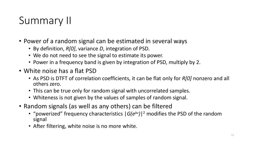
58. Summary II

• Power of a random signal can be estimated in several ways
• By definition, R[0], variance D, integration of PSD.
• We do not need to see the signal to estimate its power.
• Power in a frequency band is given by integration of PSD, multiply by 2.
• White noise has a flat PSD
• As PSD is DTFT of correlation coefficients, it can be flat only for R[0] nonzero and all
others zero.
• This can be true only for random signal with uncorrelated samples.
• Whiteness is not given by the values of samples of random signal.
• Random signals (as well as any others) can be filtered
• “powerized” frequency characteristics |G(ejω)|2 modifies the PSD of the random
signal
• After filtering, white noise is no more white.
58

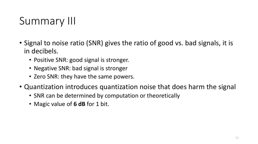
59. Summary III

• Signal to noise ratio (SNR) gives the ratio of good vs. bad signals, it is
in decibels.
• Positive SNR: good signal is stronger.
• Negative SNR: bad signal is stronger
• Zero SNR: they have the same powers.
• Quantization introduces quantization noise that does harm the signal
• SNR can be determined by computation or theoretically
• Magic value of 6 dB for 1 bit.
59