6286391

1.

Modeling the probability
of a binary outcome
Alla Stolyarevska
The Eastern-Ukrainian Branch of the International
Solomon University,
Kharkov, Ukraine
1

2.

The annotation
Now we are seeing a growing interest in machine learning as an
integral part of the discipline artificial intelligence. Some of ideas of
machine learning are raised in the course of artificial intelligence.
Machine learning is a scientific discipline concerned with the
design and development of algorithms that allow computers to evolve
behaviors based on empirical data, such as from sensor data
or databases. Data can be seen as examples that illustrate relations
between observed variables.
A learner can take advantage of data to capture characteristics of
interest of their unknown underlying probability distribution.
A major focus of machine learning research is to automatically
learn to recognize complex patterns and make intelligent decisions
based on data.
2

3.

Supervised and unsupervised learning
models
Machine learning algorithms can be organized into a taxonomy based
on the desired outcome of the algorithm.
Supervised learning generates a function that maps
inputs to desired outputs. For example, in a classification
problem, the learner approximates a function mapping a
vector into classes by looking at input-output examples of
the function.
Unsupervised learning models a set of inputs, like
clustering.
We consider the supervised learning model.
3

4.

The prerequisites for the course
The study of various aspects of machine learning requires
considerable mathematical training.
The prerequisites for this course are:
linear algebra,
nonlinear programming,
and probability
at a level expected of junior or senior undergraduate in science,
engineering or mathematics.
4

5.

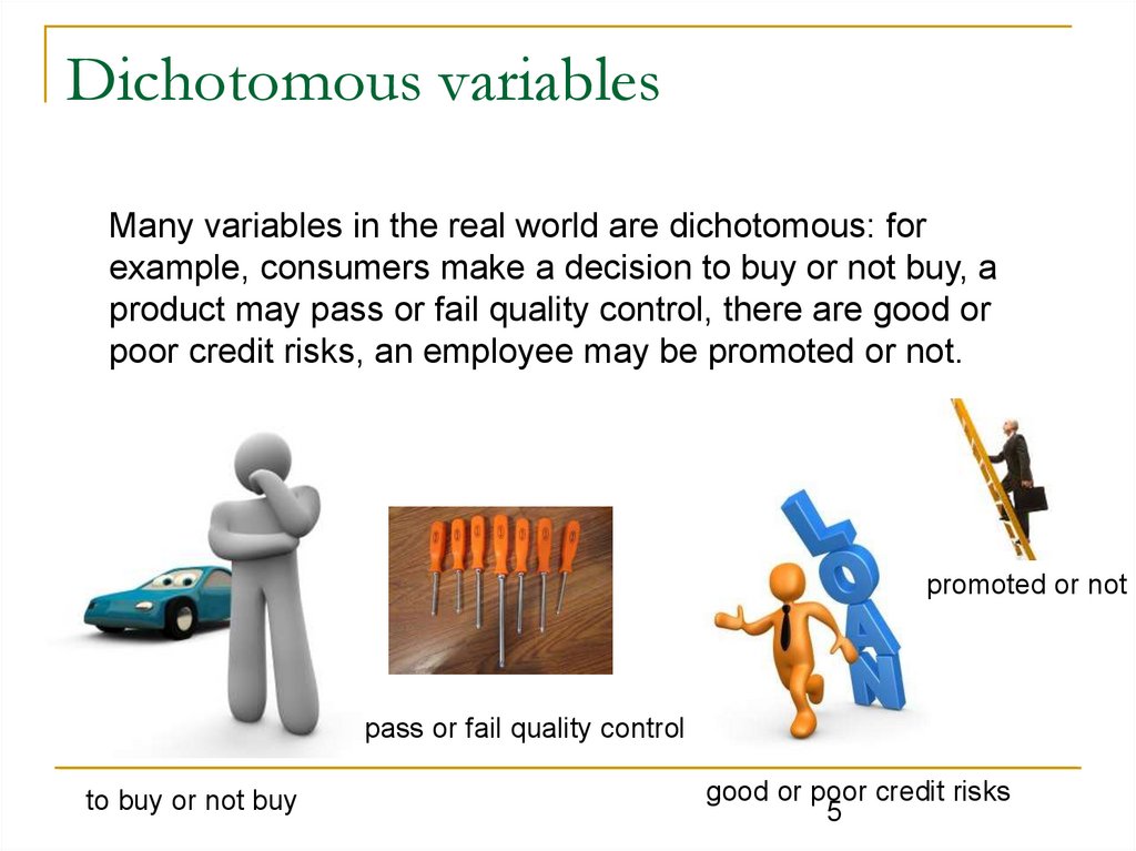
Dichotomous variables
Many variables in the real world are dichotomous: for
example, consumers make a decision to buy or not buy, a
product may pass or fail quality control, there are good or
poor credit risks, an employee may be promoted or not.
promoted or not
pass or fail quality control
to buy or not buy
good or poor credit risks
5

6.

The binary outcomes
We looked at the situation where we have a vector of input features X ,
and we want to predict a binary class Y.
The examples:
Email: Spam /NotSpam?
Online Transactions: Fraudulent (Yes/No)?
Tumor: Malignant / Benign?
y {0,1}
0: “Negative Class”
1: “Positive Class”
We’ll make the classes Y = 1, Y = 0.
Logistic Regression Model
Logistic regression. Determines the impact of multiple independent
variables presented simultaneously to predict membership of one or
other of the two dependent variable categories.
6

7.

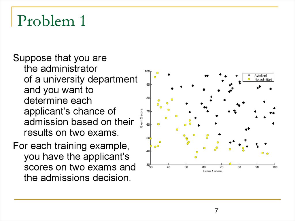
Problem 1
Suppose that you are
the administrator
of a university department
and you want to
determine each
applicant's chance of
admission based on their
results on two exams.
For each training example,
you have the applicant's
scores on two exams and
the admissions decision.
7

8.

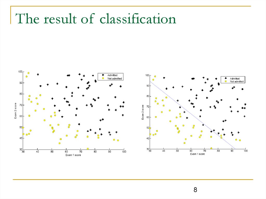
The result of classification
8

9.

Can we use linear regression on this
problem?
A linear classifier doesn't give us probabilities for the classes in
any particular case. But we've seen that we often want such
probabilities - to handle different error costs between classes, or to give
us some indication of confidence for bet-hedging, or when perfect
classification isn't possible.
If we want to estimate probabilities, we fit a stochastic model.
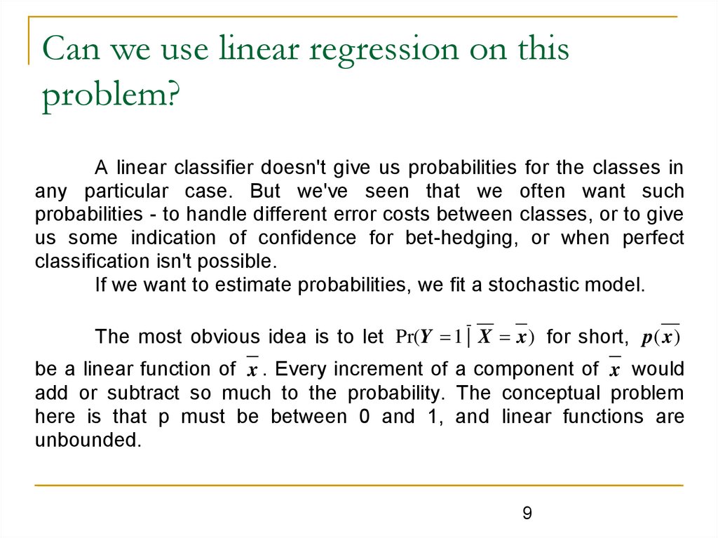
The most obvious idea is to let Pr(Y 1 | X x ) for short, p( x )
be a linear function of x . Every increment of a component of x would
add or subtract so much to the probability. The conceptual problem
here is that p must be between 0 and 1, and linear functions are
unbounded.
9

10.

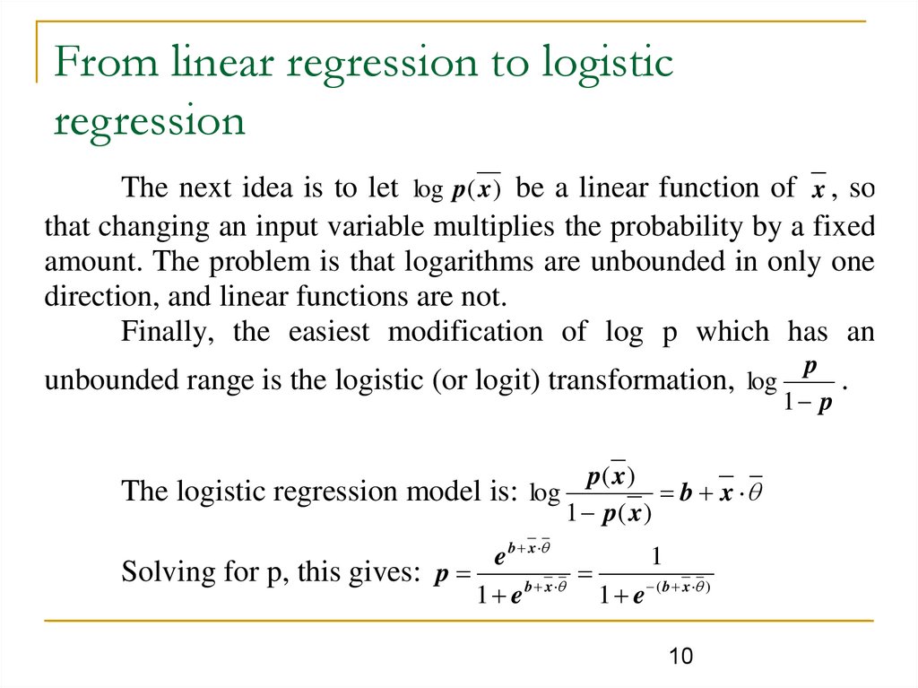
From linear regression to logistic
regression
The next idea is to let log p( x ) be a linear function of x , so
that changing an input variable multiplies the probability by a fixed
amount. The problem is that logarithms are unbounded in only one
direction, and linear functions are not.
Finally, the easiest modification of log p which has an
unbounded range is the logistic (or logit) transformation, log
The logistic regression model is: log
p( x )
b x
1 p( x )
e b x
1
Solving for p, this gives: p
1 e b x 1 e ( b x )
10
p
.
1 p

11.

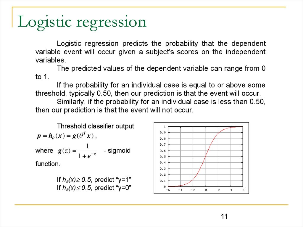
Logistic regression
Logistic regression predicts the probability that the dependent
variable event will occur given a subject's scores on the independent
variables.
The predicted values of the dependent variable can range from 0
to 1.
If the probability for an individual case is equal to or above some
threshold, typically 0.50, then our prediction is that the event will occur.
Similarly, if the probability for an individual case is less than 0.50,
then our prediction is that the event will not occur.
Threshold classifier output
p h ( x ) g ( T x ) ,
where g ( z )
1
1 e z
- sigmoid
function.
If h (x) 0.5, predict “y=1”
If h (x) 0.5, predict “y=0”
11

12.

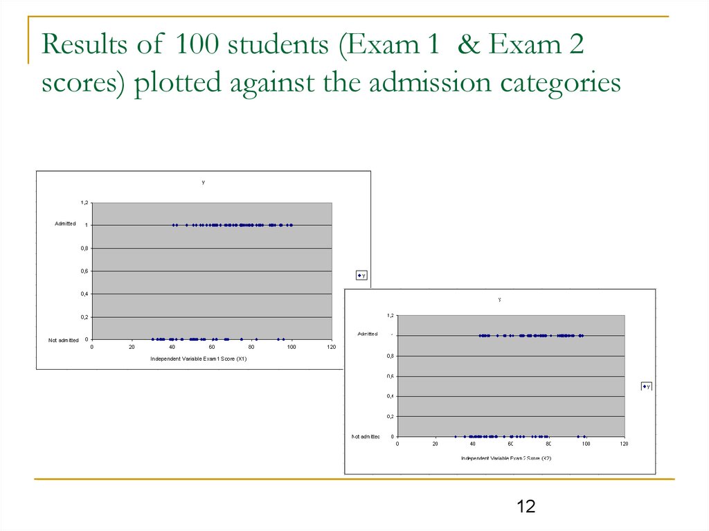
Results of 100 students (Exam 1 & Exam 2
scores) plotted against the admission categories
12

13.

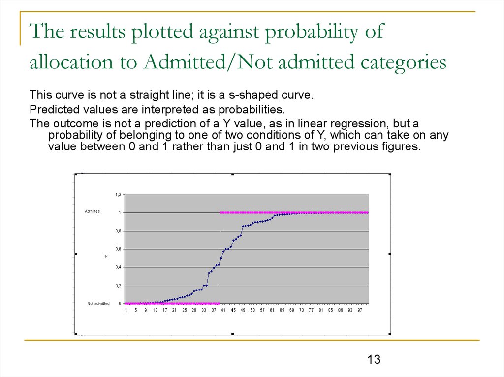
The results plotted against probability of
allocation to Admitted/Not admitted categories
This curve is not a straight line; it is a s-shaped curve.
Predicted values are interpreted as probabilities.
The outcome is not a prediction of a Y value, as in linear regression, but a
probability of belonging to one of two conditions of Y, which can take on any
value between 0 and 1 rather than just 0 and 1 in two previous figures.
13

14.

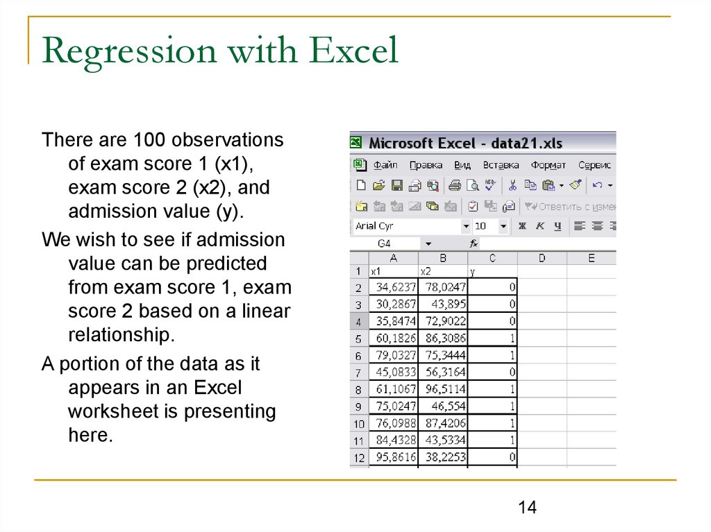
Regression with Excel
There are 100 observations
of exam score 1 (x1),
exam score 2 (x2), and
admission value (y).
We wish to see if admission
value can be predicted
from exam score 1, exam
score 2 based on a linear
relationship.
A portion of the data as it
appears in an Excel
worksheet is presenting
here.
14

15.

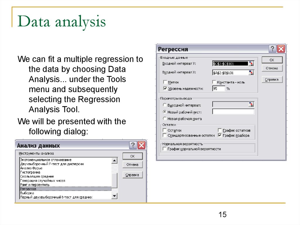
Data analysis
We can fit a multiple regression to
the data by choosing Data
Analysis... under the Tools
menu and subsequently
selecting the Regression
Analysis Tool.
We will be presented with the
following dialog:
15

16.

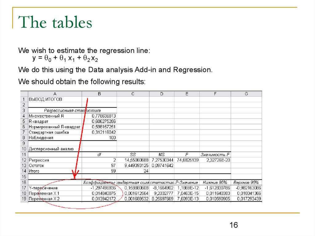
The tables
We wish to estimate the regression line:
y = 0 + 1 x1 + 2 x2
We do this using the Data analysis Add-in and Regression.
We should obtain the following results:
16

17.

Interpretation of the regression
coefficients
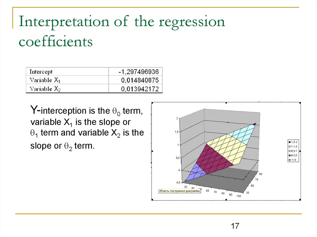
Y-interception is the 0 term,
variable X1 is the slope or
1 term and variable X2 is the
slope or 2 term.
17

18.

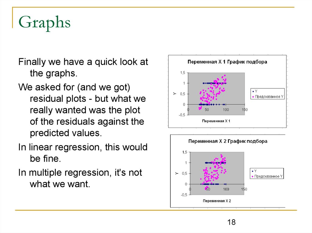
Graphs
Finally we have a quick look at
the graphs.
We asked for (and we got)
residual plots - but what we
really wanted was the plot
of the residuals against the
predicted values.
In linear regression, this would
be fine.
In multiple regression, it's not
what we want.
18

19.

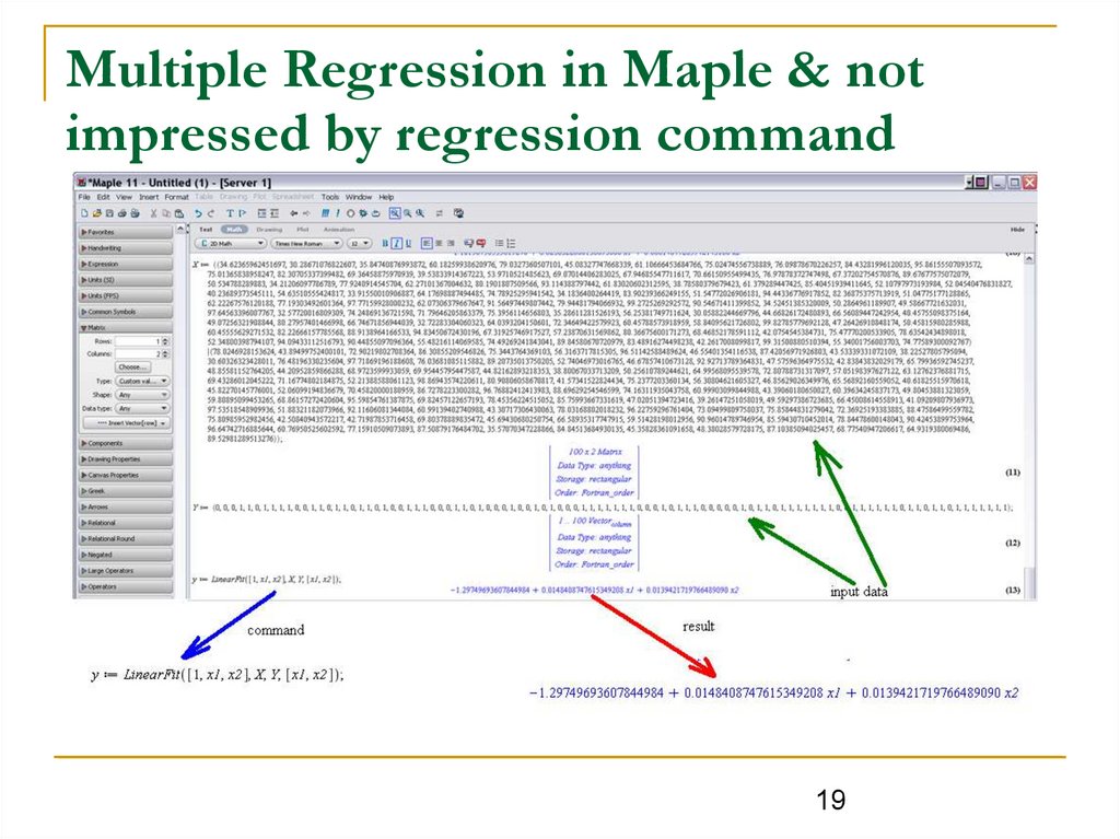
Multiple Regression in Maple & not
impressed by regression command
19

20.

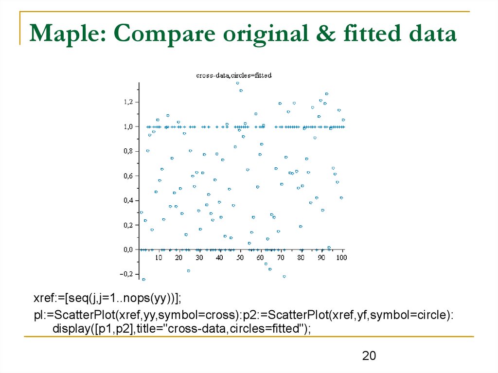
Maple: Compare original & fitted data
xref:=[seq(j,j=1..nops(yy))];
pl:=ScatterPlot(xref,yy,symbol=cross):p2:=ScatterPlot(xref,yf,symbol=circle):
display([p1,p2],title="cross-data,circles=fitted");
20

21.

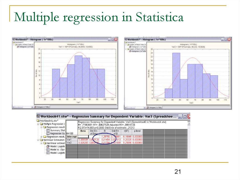
Multiple regression in Statistica
21

22.

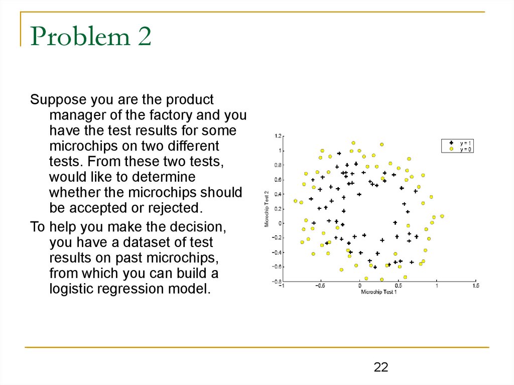
Problem 2
Suppose you are the product
manager of the factory and you
have the test results for some
microchips on two different
tests. From these two tests,
would like to determine
whether the microchips should
be accepted or rejected.
To help you make the decision,
you have a dataset of test
results on past microchips,
from which you can build a
logistic regression model.
22

23.

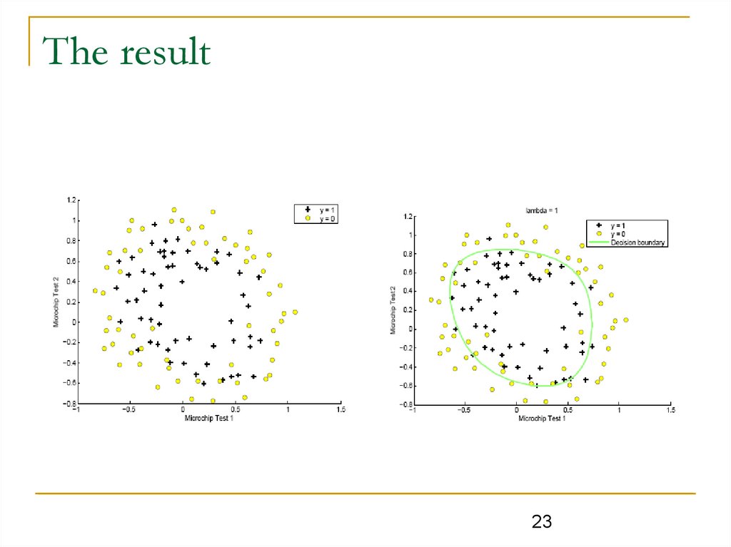
The result
23

24.

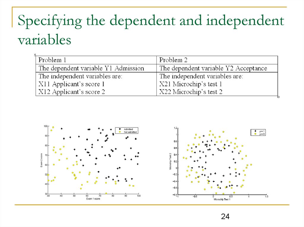
Specifying the dependent and independent
variables
24

25.

Assumptions of logistic regression
Logistic regression does not assume a linear relationship
between the dependent and independent variables.
The dependent variable must be a dichotomy
(2 categories).
The independent variables need not be interval, nor
normally distributed, nor linearly related, nor of equal variance within
each group.
The categories (groups) must be mutually exclusive and
exhaustive; a case can only be in one group and every case must be a
member of one of the groups.
Larger samples are needed than for linear regression
because maximum likelihood coefficients are large sample estimates.
A minimum of 50 cases per predictor is recommended.
25

26.

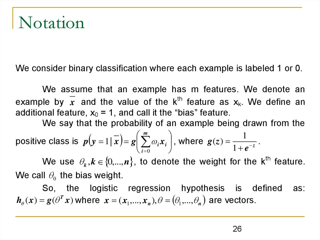
Notation
We consider binary classification where each example is labeled 1 or 0.
We assume that an example has m features. We denote an
example by x and the value of the kth feature as xk. We define an
additional feature, x0 = 1, and call it the “bias” feature.
We say that the probability of an example being drawn from the
m
1
positive class is p y 1 | x g i xi , where g ( z )
.
z
1 e
i 0
We use k , k 0,..., n , to denote the weight for the kth feature.
We call 0 the bias weight.
So, the logistic regression hypothesis is defined
h ( x ) g ( T x ) where x ( x1 ,..., xn ), 1 ,..., n are vectors.
26
as:

27.

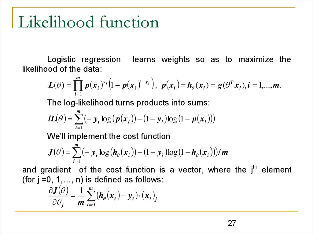
Likelihood function
Logistic regression
likelihood of the data:
m
learns weights so as to maximize the
L( ) p xi i 1 p xi
y
1 y i
, p x h ( x ) g( x ), i 1,..., m.
i
T
i
i
i 1
The log-likelihood turns products into sums:
m
lL yi log p xi 1 yi log 1 p xi
i 1
We’ll implement the cost function
m
J yi log h xi 1 yi log 1 h xi / m
i 1
and gradient of the cost function is a vector, where the jth element
(for j =0, 1,…, n) is defined as follows:
J 1 m
h xi yi xi j
j
m i 0
27

28.

Numerical optimization
There are a huge number of methods for numerical
optimization; we can't cover all bases, and there is no magical method
which will always work better than anything else. However, there are
some methods which work very well on an awful lot of the problems
which keep coming up, and it's worth spending a moment to sketch
how they work.
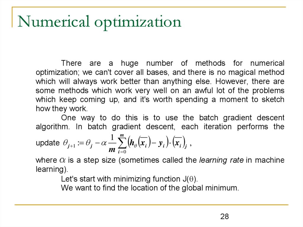
One way to do this is to use the batch gradient descent
algorithm. In batch gradient descent, each iteration performs the
1 m
update j 1 : j h xi yi xi j ,
m i 0
where is a step size (sometimes called the learning rate in machine
learning).
Let's start with minimizing function J( ).
We want to find the location of the global minimum.
28

29.

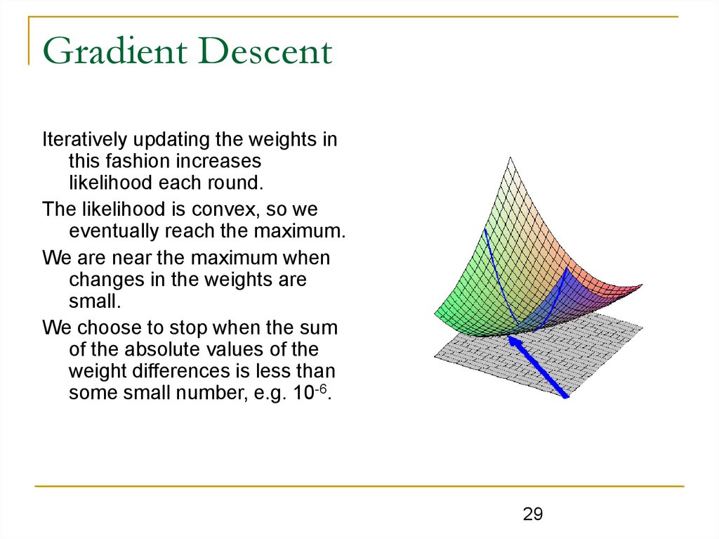
Gradient Descent
Iteratively updating the weights in
this fashion increases
likelihood each round.
The likelihood is convex, so we
eventually reach the maximum.
We are near the maximum when
changes in the weights are
small.
We choose to stop when the sum
of the absolute values of the
weight differences is less than
some small number, e.g. 10-6.
29

30.

Octave
GNU Octave is a high-level interpreted
language, primarily intended for
numerical computations.
It provides capabilities for the numerical
solution of linear and nonlinear
problems, and for performing other
numerical experiments.
It also provides extensive graphics
capabilities for data visualization
and manipulation.
Octave is normally used through its
interactive command line interface,
but it can also be used to write noninteractive programs.
Octave is distributed under the terms of
the GNU General Public License.
30

31.

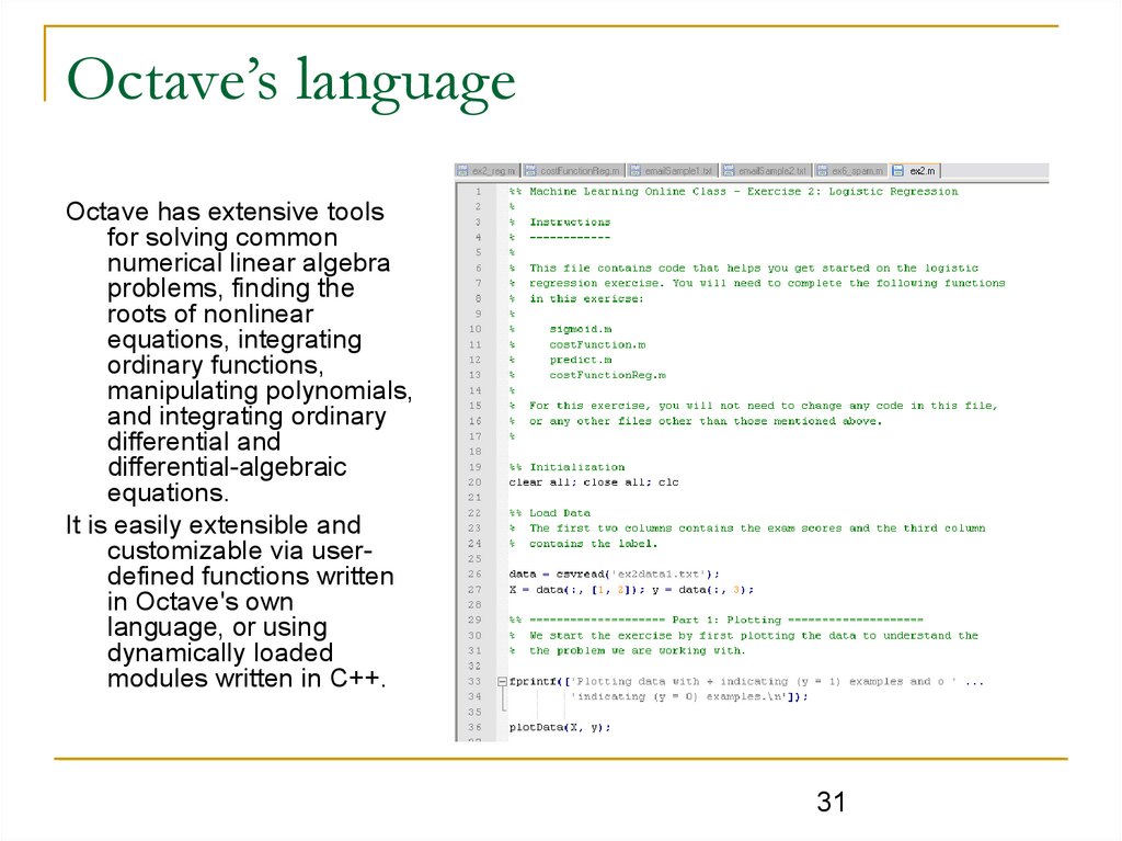
Octave’s language
Octave has extensive tools
for solving common
numerical linear algebra
problems, finding the
roots of nonlinear
equations, integrating
ordinary functions,
manipulating polynomials,
and integrating ordinary
differential and
differential-algebraic
equations.
It is easily extensible and
customizable via userdefined functions written
in Octave's own
language, or using
dynamically loaded
modules written in C++.
31

32.

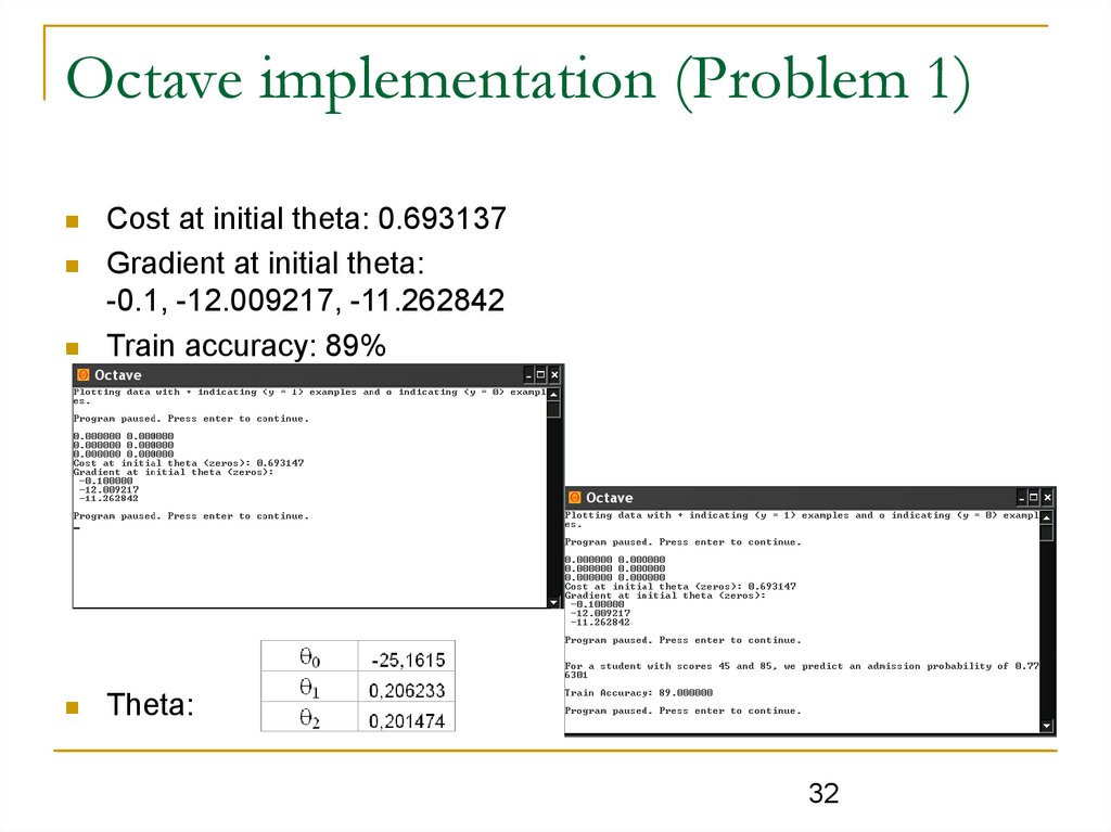
Octave implementation (Problem 1)
Cost at initial theta: 0.693137
Gradient at initial theta:
-0.1, -12.009217, -11.262842
Train accuracy: 89%
Theta:
32

33.

Evaluating logistic regression
(Problem 1, prediction)
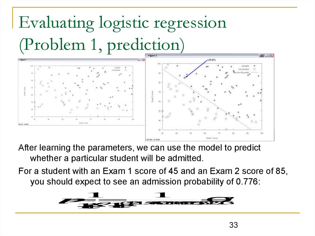
After learning the parameters, we can use the model to predict
whether a particular student will be admitted.
For a student with an Exam 1 score of 45 and an Exam 2 score of 85,
you should expect to see an admission probability of 0.776:
1
1
p
0
.
7763
(
1
*
25
.
161537
45
*
0
.
206233
85
*
0
.
201474
)
x
1
e
1
e
33

34.

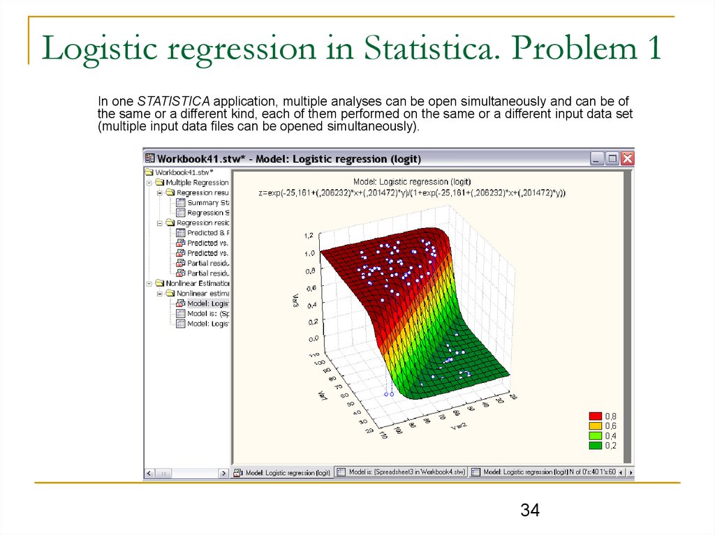
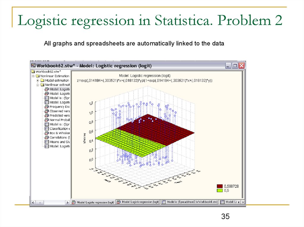
Logistic regression in Statistica. Problem 1
In one STATISTICA application, multiple analyses can be open simultaneously and can be of
the same or a different kind, each of them performed on the same or a different input data set
(multiple input data files can be opened simultaneously).
34

35.

Logistic regression in Statistica. Problem 2
All graphs and spreadsheets are automatically linked to the data
35

36.

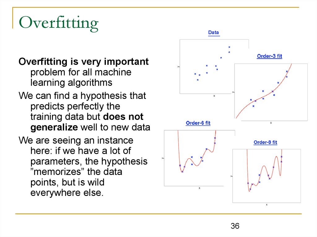
Overfitting
Overfitting is very important
problem for all machine
learning algorithms
We can find a hypothesis that
predicts perfectly the
training data but does not
generalize well to new data
We are seeing an instance
here: if we have a lot of
parameters, the hypothesis
”memorizes” the data
points, but is wild
everywhere else.
36

37.

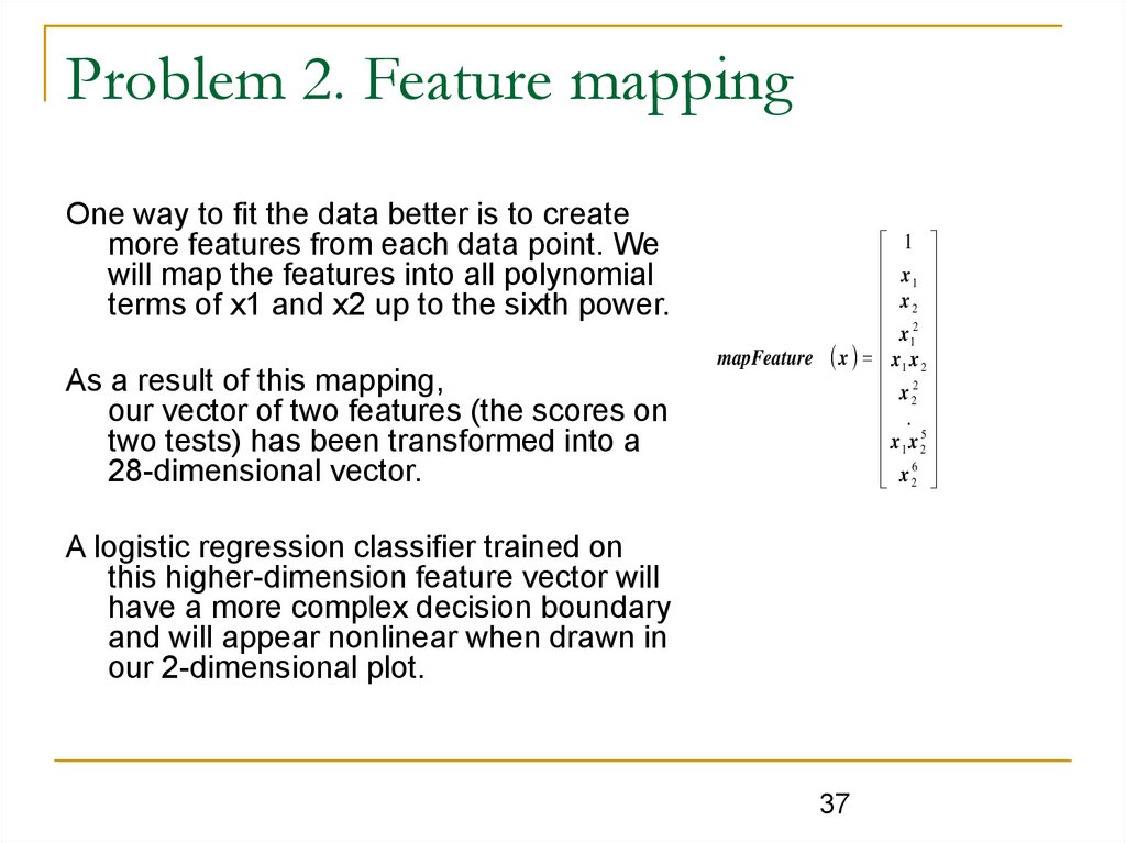
Problem 2. Feature mapping
One way to fit the data better is to create
more features from each data point. We
will map the features into all polynomial
terms of x1 and x2 up to the sixth power.
As a result of this mapping,
our vector of two features (the scores on
two tests) has been transformed into a
28-dimensional vector.
1
x
1
x2
x2
1
mapFeature x x1 x 2
x 22
.
x x5
1 62
x 2
A logistic regression classifier trained on
this higher-dimension feature vector will
have a more complex decision boundary
and will appear nonlinear when drawn in
our 2-dimensional plot.
37

38.

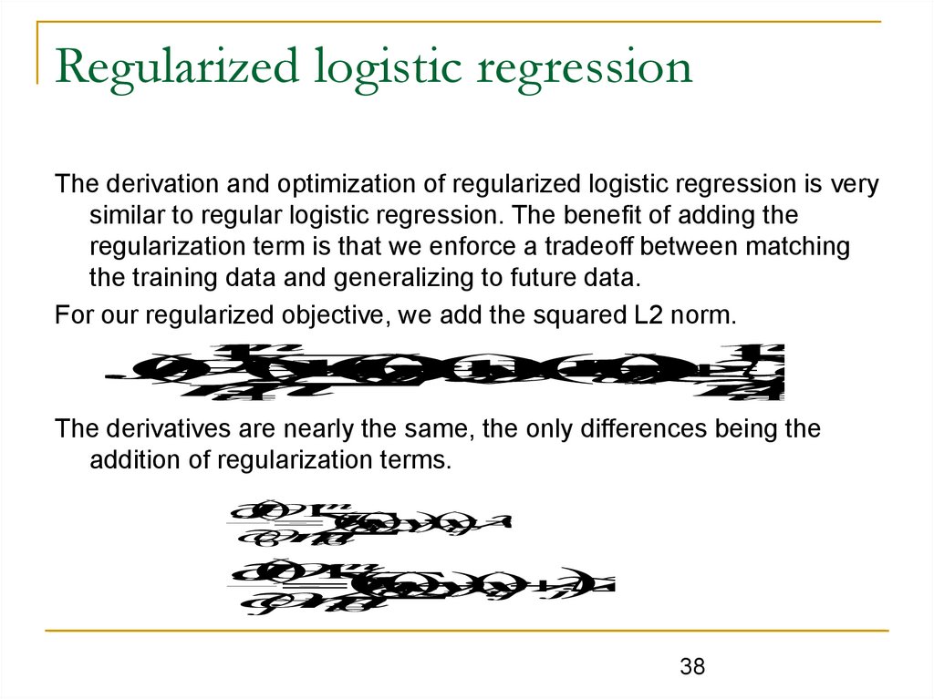
Regularized logistic regression
The derivation and optimization of regularized logistic regression is very
similar to regular logistic regression. The benefit of adding the
regularization term is that we enforce a tradeoff between matching
the training data and generalizing to future data.
For our regularized objective, we add the squared L2 norm.
m
n
1
1
2
J
y
log
h
x
1
y
log
1
h
x
i
i
i
i
i
m
2
m
i
1
i
1
The derivatives are nearly the same, the only differences being the
addition of regularization terms.
m
J
1
h
x
y
x
,
0
i
i
i
j
m
i
0
0
m
J
1
h
x
y
x
,
1
i
i
i
j
j
m
i
0
j
38

39.

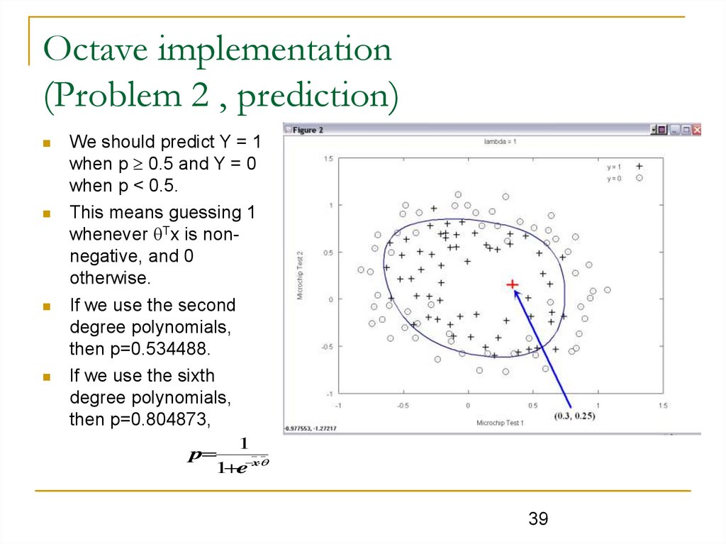
Octave implementation
(Problem 2 , prediction)
We should predict Y = 1
when p 0.5 and Y = 0
when p < 0.5.
This means guessing 1
whenever Tx is nonnegative, and 0
otherwise.
If we use the second
degree polynomials,
then p=0.534488.
If we use the sixth
degree polynomials,
then p=0.804873,
1
p
1 e x
39

40.

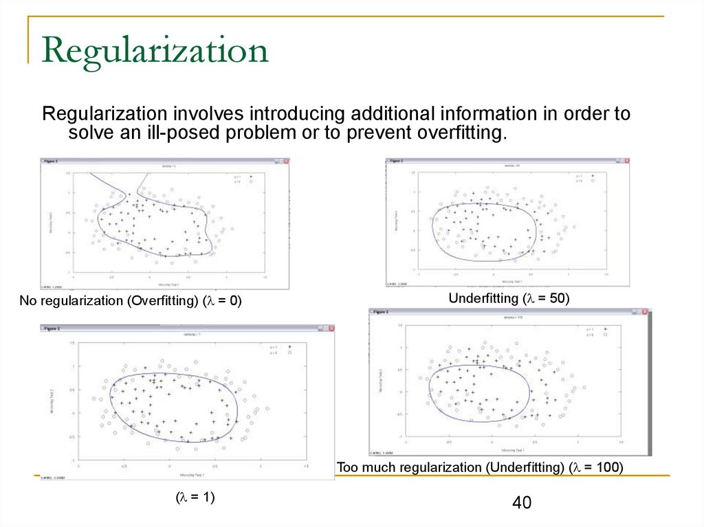
Regularization
Regularization involves introducing additional information in order to
solve an ill-posed problem or to prevent overfitting.
No regularization (Overfitting) ( = 0)
Underfitting ( = 50)
Too much regularization (Underfitting) ( = 100)
( = 1)
40

41.

Model accuracy
A way to test for errors in models created by step-wise regression is
to not rely on the model's F-statistic, significance, or multiple-r,
but instead assess the model against a set of data that was not
used to create the model. The class of techniques is called
cross-validation.
Accuracy is measured as correctly classified records in the holdout
sample. There are four possible classifications:
prediction of 0 when the holdout sample has a 0
True Negative/TN
prediction of 0 when the holdout sample has a 1
False Negative/FN
prediction of 1 when the holdout sample has a 0
False Positive/FP
prediction of 1 when the holdout sample has a 1
True Positive/TP
41

42.

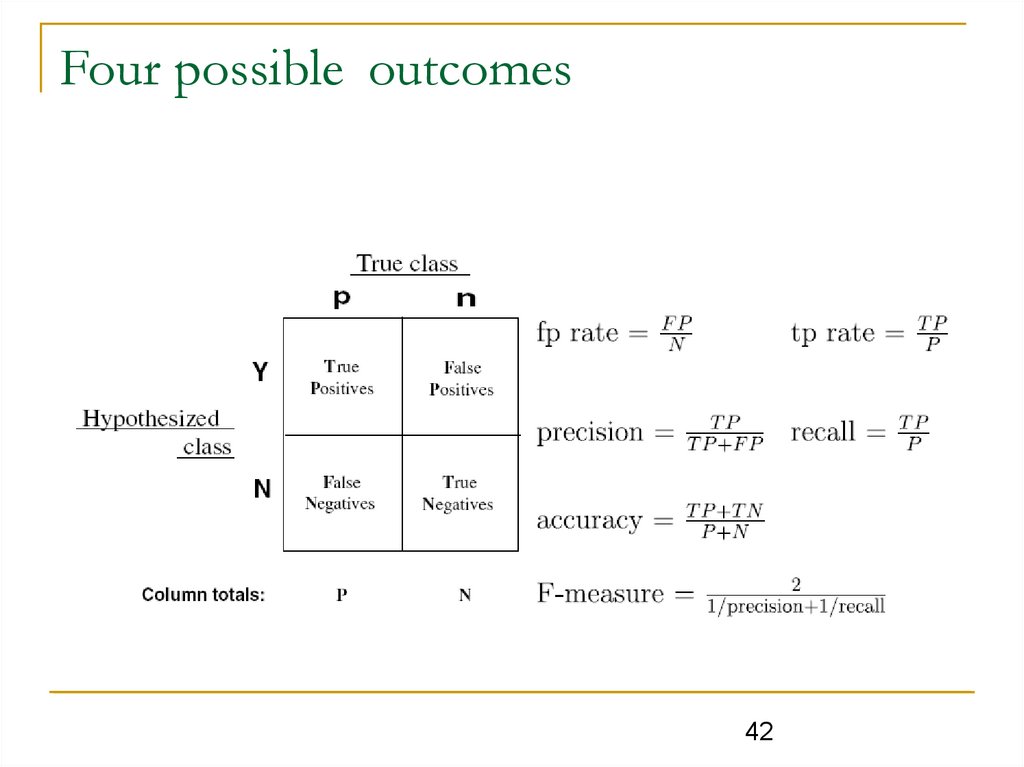
Four possible outcomes
42

43.

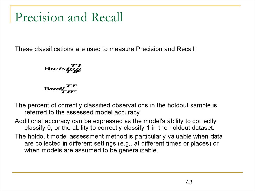
Precision and Recall
These classifications are used to measure Precision and Recall:
TP
Pr
ecision
TP
FP
TP
Re
call
TP
FN
The percent of correctly classified observations in the holdout sample is
referred to the assessed model accuracy.
Additional accuracy can be expressed as the model's ability to correctly
classify 0, or the ability to correctly classify 1 in the holdout dataset.
The holdout model assessment method is particularly valuable when data
are collected in different settings (e.g., at different times or places) or
when models are assumed to be generalizable.
43

44.

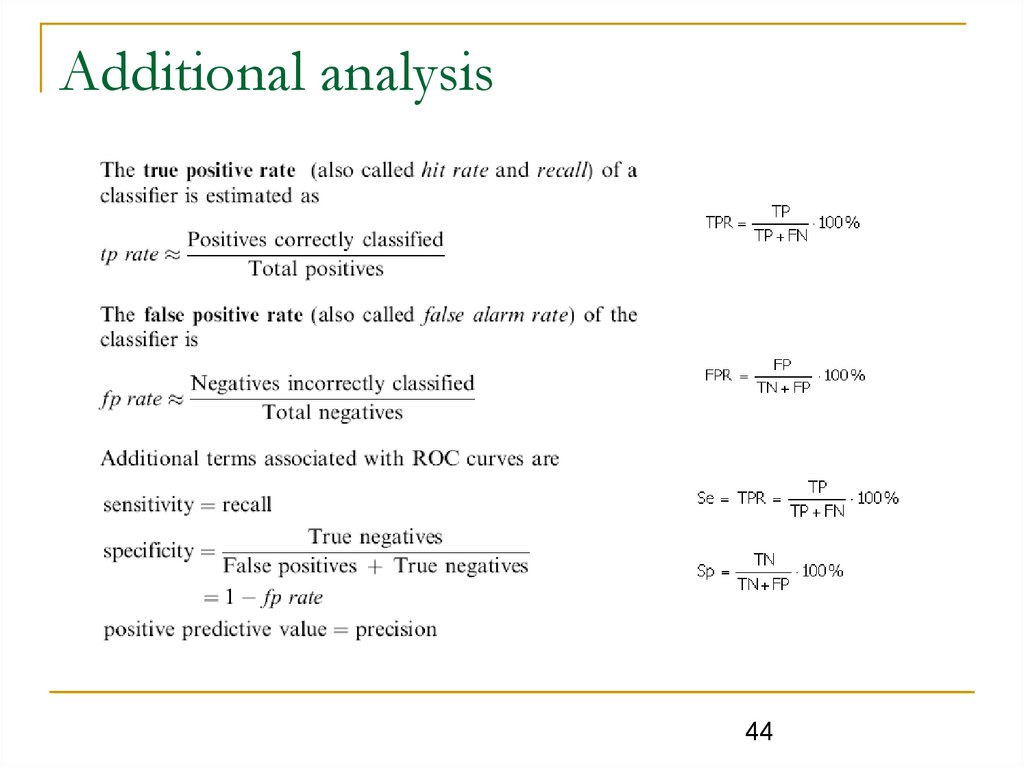
Additional analysis
44

45.

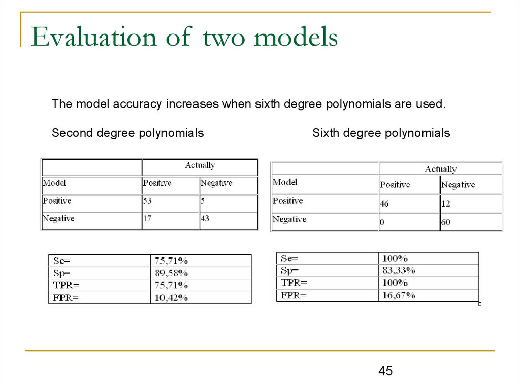
Evaluation of two models
The model accuracy increases when sixth degree polynomials are used.
Second degree polynomials
Sixth degree polynomials
45

46.

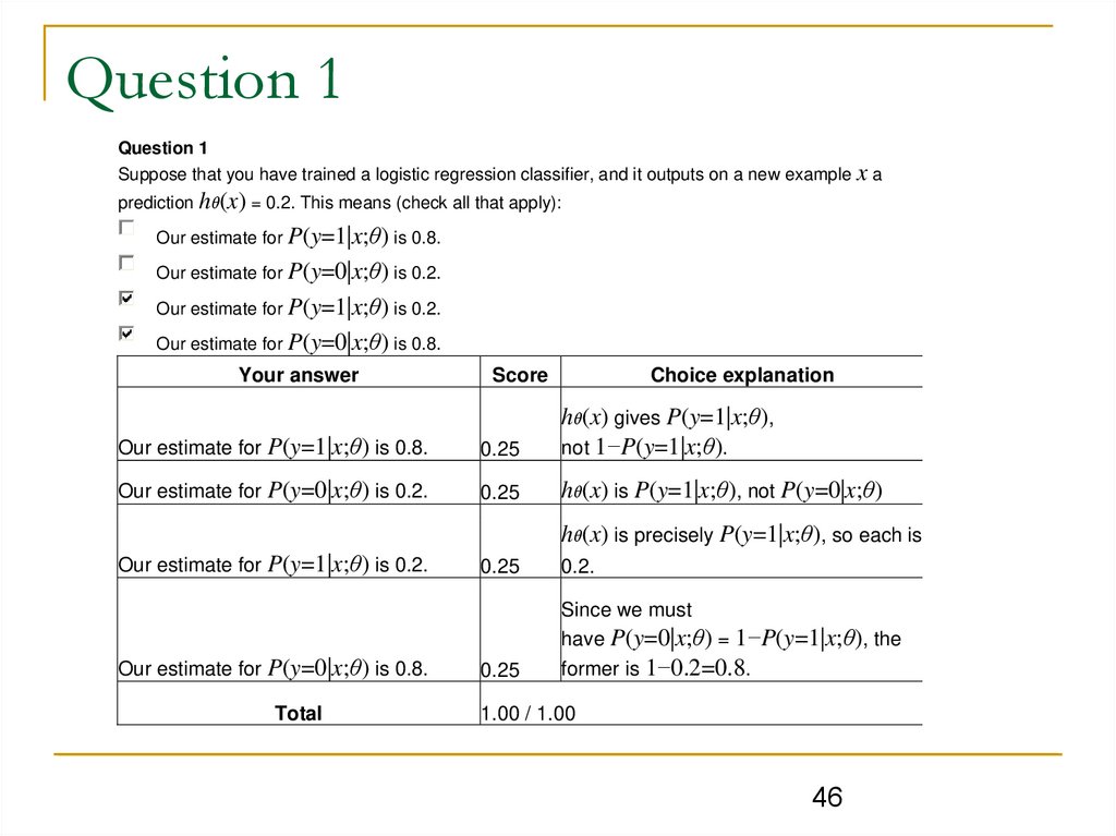
Question 1
Question 1
Suppose that you have trained a logistic regression classifier, and it outputs on a new example x a
prediction hθ(x) = 0.2. This means (check all that apply):
Our estimate for P(y=1|x;θ) is 0.8.
Our estimate for P(y=0|x;θ) is 0.2.
Our estimate for P(y=1|x;θ) is 0.2.
Our estimate for P(y=0|x;θ) is 0.8.
Your answer
Score
Choice explanation
Our estimate for P(y=1|x;θ) is 0.8.
0.25
hθ(x) gives P(y=1|x;θ),
not 1−P(y=1|x;θ).
Our estimate for P(y=0|x;θ) is 0.2.
0.25
hθ(x) is P(y=1|x;θ), not P(y=0|x;θ)
hθ(x) is precisely P(y=1|x;θ), so each is
Our estimate for P(y=1|x;θ) is 0.2.
Our estimate for P(y=0|x;θ) is 0.8.
Total
0.25
0.2.
0.25
Since we must
have P(y=0|x;θ) = 1−P(y=1|x;θ), the
former is 1−0.2=0.8.
1.00 / 1.00
46

47.

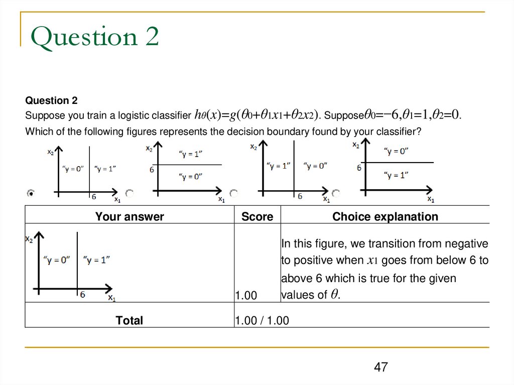
Question 2
Question 2
Suppose you train a logistic classifier hθ(x)=g(θ0+θ1x1+θ2x2). Supposeθ0=−6,θ1=1,θ2=0.
Which of the following figures represents the decision boundary found by your classifier?
Your answer
Choice explanation
Score
In this figure, we transition from negative
to positive when x1 goes from below 6 to
1.00
Total
above 6 which is true for the given
values of θ.
1.00 / 1.00
47

48.

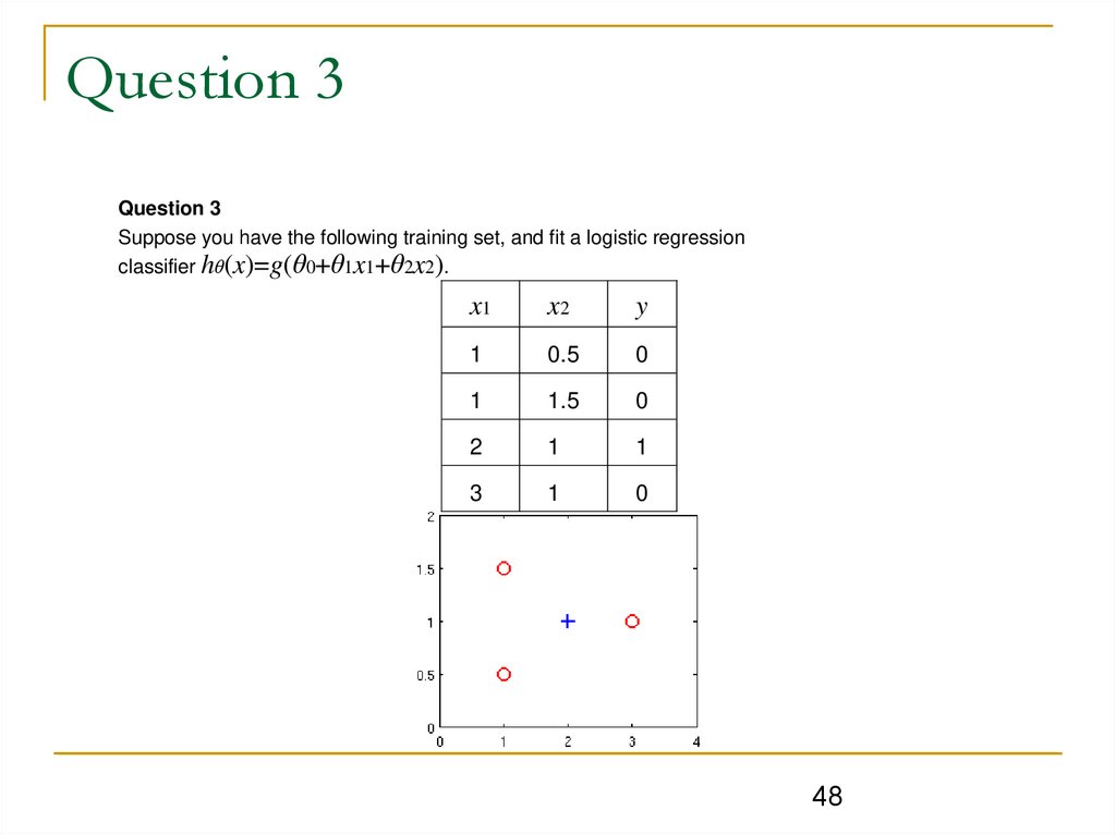
Question 3
Question 3
Suppose you have the following training set, and fit a logistic regression
classifier hθ(x)=g(θ0+θ1x1+θ2x2).
x1
x2
y
1
0.5
0
1
1.5
0
2
1
1
3
1
0
48

49.

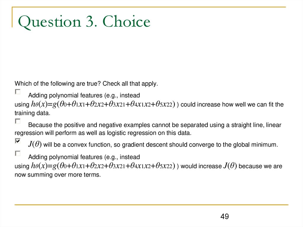
Question 3. Choice
Which of the following are true? Check all that apply.
Adding polynomial features (e.g., instead
using hθ(x)=g(θ0+θ1x1+θ2x2+θ3x21+θ4x1x2+θ5x22) ) could increase how well we can fit the
training data.
Because the positive and negative examples cannot be separated using a straight line, linear
regression will perform as well as logistic regression on this data.
J(θ) will be a convex function, so gradient descent should converge to the global minimum.
Adding polynomial features (e.g., instead
using hθ(x)=g(θ0+θ1x1+θ2x2+θ3x21+θ4x1x2+θ5x22) ) would increase J(θ) because we are
now summing over more terms.
49

50.

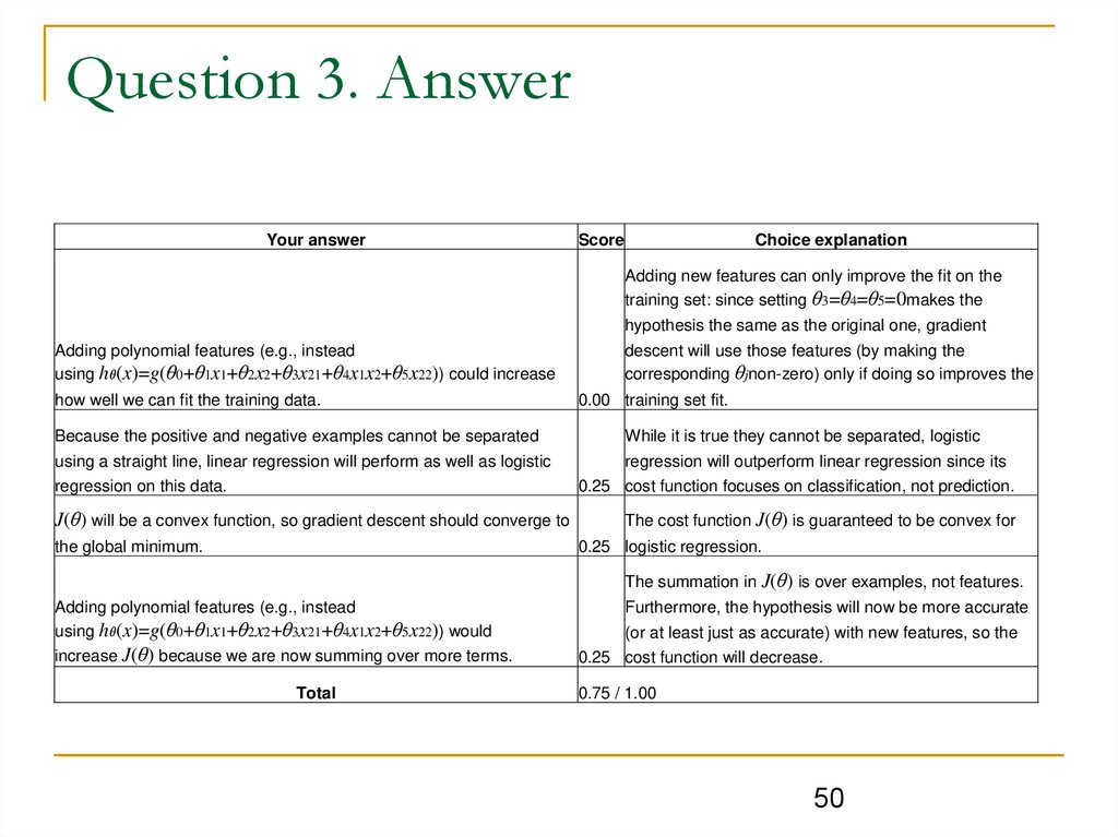
Question 3. Answer
Your answer
Choice explanation
Score
Adding new features can only improve the fit on the
training set: since setting θ3=θ4=θ5=0makes the
Adding polynomial features (e.g., instead
using hθ(x)=g(θ0+θ1x1+θ2x2+θ3x21+θ4x1x2+θ5x22)) could increase
how well we can fit the training data.
Because the positive and negative examples cannot be separated
using a straight line, linear regression will perform as well as logistic
hypothesis the same as the original one, gradient
descent will use those features (by making the
corresponding θjnon-zero) only if doing so improves the
0.00 training set fit.
While it is true they cannot be separated, logistic
regression will outperform linear regression since its
0.25 cost function focuses on classification, not prediction.
regression on this data.
J(θ) will be a convex function, so gradient descent should converge to
The cost function J(θ) is guaranteed to be convex for
0.25 logistic regression.
the global minimum.
The summation in J(θ) is over examples, not features.
Adding polynomial features (e.g., instead
using hθ(x)=g(θ0+θ1x1+θ2x2+θ3x21+θ4x1x2+θ5x22)) would
increase J(θ) because we are now summing over more terms.
Total
Furthermore, the hypothesis will now be more accurate
(or at least just as accurate) with new features, so the
0.25 cost function will decrease.
0.75 / 1.00
50

51.

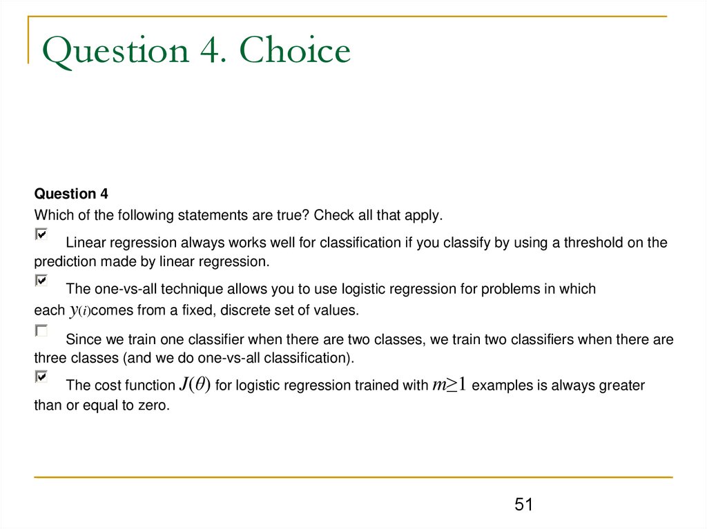
Question 4. Choice
Question 4
Which of the following statements are true? Check all that apply.
Linear regression always works well for classification if you classify by using a threshold on the
prediction made by linear regression.
The one-vs-all technique allows you to use logistic regression for problems in which
each y(i)comes from a fixed, discrete set of values.
Since we train one classifier when there are two classes, we train two classifiers when there are
three classes (and we do one-vs-all classification).
The cost function J(θ) for logistic regression trained with m≥1 examples is always greater
than or equal to zero.
51

52.

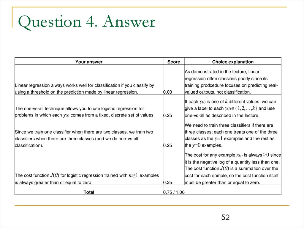
Question 4. Answer
Your answer
Score
Choice explanation
As demonstrated in the lecture, linear
regression often classifies poorly since its
Linear regression always works well for classification if you classify by
using a threshold on the prediction made by linear regression.
The one-vs-all technique allows you to use logistic regression for
problems in which each y(i) comes from a fixed, discrete set of values.
training prodcedure focuses on predicting real0.00
valued outputs, not classification.
If each y(i) is one of k different values, we can
give a label to each y(i) {1,2,…,k} and use
0.25
one-vs-all as described in the lecture.
We need to train three classifiers if there are
Since we train one classifier when there are two classes, we train two
classifiers when there are three classes (and we do one-vs-all
classification).
three classes; each one treats one of the three
classes as the y=1 examples and the rest as
0.25
the y=0 examples.
The cost for any example x(i) is always ≥0 since
it is the negative log of a quantity less than one.
The cost function J(θ) is a summation over the
The cost function J(θ) for logistic regression trained with m≥1 examples
is always greater than or equal to zero.
Total
0.25
cost for each eample, so the cost function itself
must be greater than or equal to zero.
0.75 / 1.00
52

53.

Questions 5-10
Qu. 5
Why are p values transformed to a log value in logistic regression?
(a) because p values are extremely small
(b) because p values cannot be analyzed
(c) because p values only range between 0 and 1
(d) because p values are not normally distributed
(e) none of the above
Qu. 6
Logistic regression is based on:
(a) normal distribution
(b) Poisson distribution
(c) the sine curve
(d) binomial distribution
Qu. 7
Logistic regression is essential where,
(a) both the dependent variable and independent variable(s) are interval
(b) the independent variable is interval and both the dependent variables are
categorical
(c) the sole dependent variable is categorical and the independent variable is not
interval
(d) there is only one dependent variable irrespective of the number or type of the
independent variable(s)
Qu. 8
Explain briefly why a line of best fit approach cannot be applied in logistic regression.
Check your response in the material above.
Qu. 9
Under what circumstances would you choose to use logistic regression?
Check your response with the material above.
Qu. 10
What is the probability that a student, which passed two exams with results 50, 48, will
be admitted.
Check your answer.
53

54.

Results
Text
54

55.

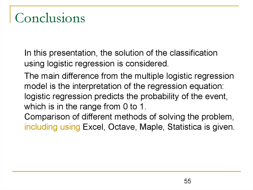
Conclusions
In this presentation, the solution of the classification
using logistic regression is considered.
The main difference from the multiple logistic regression
model is the interpretation of the regression equation:
logistic regression predicts the probability of the event,
which is in the range from 0 to 1.
Comparison of different methods of solving the problem,
including using Excel, Octave, Maple, Statistica is given.
55

56.

Thank You for attention!
56