


 warping")


Похожие презентации:


")
")


Image Stitching
1. Image Stitching
Ali FarhadiCSE 455
Several slides from Rick Szeliski, Steve Seitz, Derek Hoiem, and Ira Kemelmacher
2.
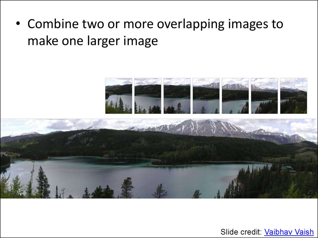
• Combine two or more overlapping images tomake one larger image
Add example
Slide credit: Vaibhav Vaish
3. How to do it?
• Basic Procedure1. Take a sequence of images from the same
position
1. Rotate the camera about its optical center
2. Compute transformation between second image
and first
3. Shift the second image to overlap with the first
4. Blend the two together to create a mosaic
5. If there are more images, repeat
4. 1. Take a sequence of images from the same position
• Rotate the camera about its optical center5. 2. Compute transformation between images
• Extract interest points• Find Matches
• Compute transformation
?
6. 3. Shift the images to overlap
7. 4. Blend the two together to create a mosaic
8. 5. Repeat for all images
9. How to do it?
• Basic Procedure✓ 1. Take a sequence of images from the same
position
1. Rotate the camera about its optical center
2. Compute transformation between second image
and first
3. Shift the second image to overlap with the first
4. Blend the two together to create a mosaic
5. If there are more images, repeat
10. Compute Transformations
✓ • Extract interest points✓ • Find good matches
• Compute transformation
Let’s assume we are given a set of good matching
interest points
11. Image reprojection
mosaic PP• The mosaic has a natural interpretation in 3D
– The images are reprojected onto a common plane
– The mosaic is formed on this plane
12. Example
Camera Center13. Image reprojection
• Observation– Rather than thinking of this as a 3D reprojection, think
of it as a 2D image warp from one image to another
14. Motion models
• What happens when we take two images witha camera and try to align them?
• translation?
• rotation?
• scale?
• affine?
• Perspective?
15. Recall: Projective transformations
• (aka homographies)16. Parametric (global) warping
• Examples of parametric warps:aspect
rotation
translation
perspective
affine
17. 2D coordinate transformations
translation: x’ = x + t
x = (x,y)
rotation: x’ = R x + t
similarity:
x’ = s R x + t
affine:
x’ = A x + t
perspective: x’ H x
x = (x,y,1)
(x is a homogeneous coordinate)
18. Image Warping
• Given a coordinate transform x’ = h(x) and asource image f(x), how do we compute a
transformed image g(x’) = f(h(x))?
h(x)
x
f(x)
x’
g(x’)
19. Forward Warping
• Send each pixel f(x) to its correspondinglocation x’ = h(x) in g(x’)
• What if pixel lands “between” two pixels?
h(x)
x
f(x)
x’
g(x’)
20. Forward Warping
• Send each pixel f(x) to its correspondinglocation x’ = h(x) in g(x’)
• What if pixel lands “between” two pixels?
• Answer: add “contribution” to several pixels,
normalize later (splatting)
h(x)
x
f(x)
x’
g(x’)
21. Inverse Warping
• Get each pixel g(x’) from its correspondinglocation x’ = h(x) in f(x)
• What if pixel comes from “between” two pixels?
h-1(x)
x
Richard Szeliski
x’
f(x)
Image Stitching
g(x’)
21
22. Inverse Warping
• Get each pixel g(x’) from its correspondinglocation x’ = h(x) in f(x)
• What if pixel comes from “between” two pixels?
• Answer: resample color value from
interpolated source image
h-1(x)
x
Richard Szeliski
x’
f(x)
Image Stitching
g(x’)
22
23. Interpolation
• Possible interpolation filters:– nearest neighbor
– bilinear
– bicubic (interpolating)
24. Motion models
TranslationAffine
Perspective
2 unknowns
6 unknowns
8 unknowns
25. Finding the transformation
Translation =
Similarity =
Affine
=
Homography
2 degrees of freedom
4 degrees of freedom
6 degrees of freedom
= 8 degrees of freedom
• How many corresponding points do we need
to solve?
26. Plane perspective mosaics
Simple case: translationsHow do we solve for
?
27. Simple case: translations
Displacement of match i =Mean displacement =
28. Simple case: translations
• System of linear equations– What are the knowns? Unknowns?
– How many unknowns? How many equations (per match)?
29. Simple case: translations
• Problem: more equations than unknowns– “Overdetermined” system of equations
– We will find the least squares solution
30. Simple case: translations
Least squares formulation• For each point
• we define the residuals as
31. Least squares formulation
• Goal: minimize sum of squared residuals• “Least squares” solution
• For translations, is equal to mean displacement
32. Least squares formulation
Least squares• Find t that minimizes
• To solve, form the normal equations
33. Least squares
Solving for translations• Using least squares
2n x 2
2x1
2n x 1
34. Solving for translations
Affine transformations• How many unknowns?
• How many equations per match?
• How many matches do we need?
35. Affine transformations
• Residuals:• Cost function:
36. Affine transformations
• Matrix form2n x 6
6x1
2n x 1
37. Affine transformations
Solving for homographies38. Solving for homographies
39. Solving for homographies
Direct Linear Transforms2n × 9
9
Defines a least squares problem:
• Since
is only defined up to scale, solve for unit vector
• Solution:
= eigenvector of
with smallest eigenvalue
• Works with 4 or more points
2n
40. Direct Linear Transforms
Matching featuresWhat do we do about the “bad” matches?
Richard Szeliski
Image Stitching
41
41. Matching features
RAndom SAmple ConsensusSelect one match, count inliers
Richard Szeliski
Image Stitching
42
42. RAndom SAmple Consensus
Select one match, count inliersRichard Szeliski
Image Stitching
43
43. RAndom SAmple Consensus
Least squares fitFind “average” translation vector
Richard Szeliski
Image Stitching
44
44. Least squares fit
45.
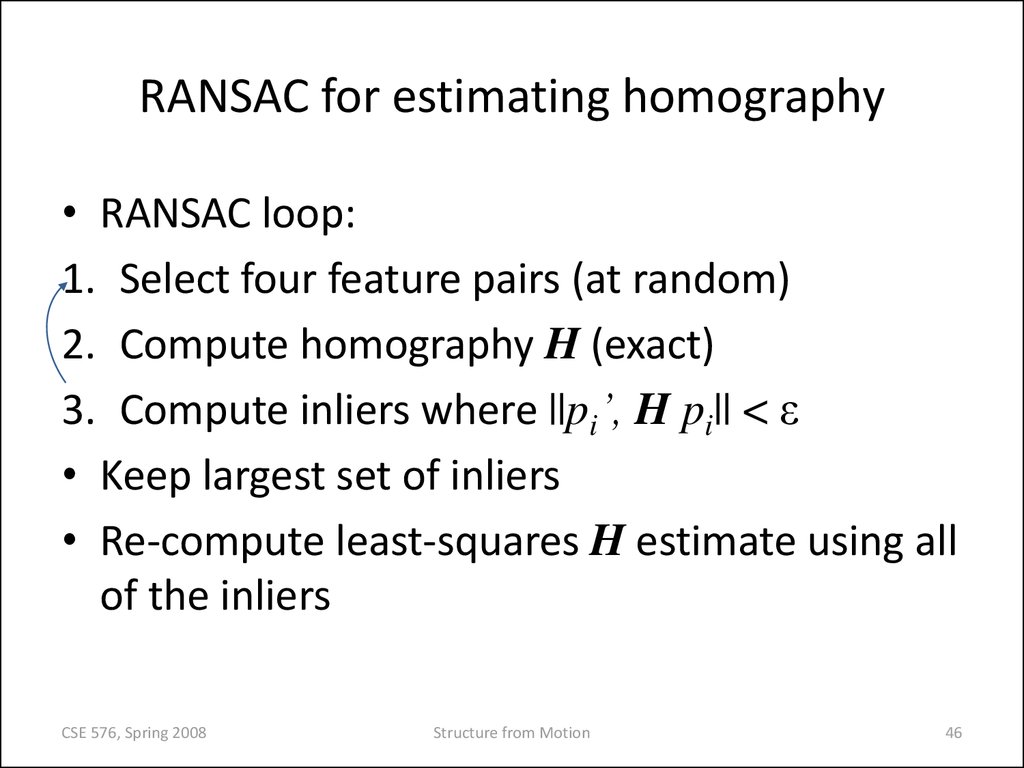
RANSAC for estimating homography• RANSAC loop:
1. Select four feature pairs (at random)
2. Compute homography H (exact)
3. Compute inliers where ||pi’, H pi|| < ε
• Keep largest set of inliers
• Re-compute least-squares H estimate using all
of the inliers
CSE 576, Spring 2008
Structure from Motion
46
46. RANSAC for estimating homography
Simple example: fit a line• Rather than homography H (8 numbers)
fit y=ax+b (2 numbers a, b) to 2D pairs
47
47
47. Simple example: fit a line
• Pick 2 points• Fit line
• Count inliers
3 inliers
48
48
48. Simple example: fit a line
• Pick 2 points• Fit line
• Count inliers
4 inliers
49
49
49. Simple example: fit a line
• Pick 2 points• Fit line
• Count inliers
9 inliers
50
50
50. Simple example: fit a line
• Pick 2 points• Fit line
• Count inliers
8 inliers
51
51
51. Simple example: fit a line
• Use biggest set of inliers• Do least-square fit
52
52
52. Simple example: fit a line
RANSACRed:
rejected by 2nd nearest neighbor criterion
Blue:
Ransac outliers
Yellow:
inliers
53. RANSAC
Computing homography• Assume we have four matched points: How do we compute
homography H?
Normalized DLT
1. Normalize coordinates for each image
a)
b)
Translate for zero mean
Scale so that average distance to origin is ~sqrt(2)
–
This makes problem better behaved numerically
~
x Tx
~x T x
~ using DLT in normalized coordinates
2. Compute H
~
3. Unnormalize: H T 1H
T
x i Hx i
54. How many rounds?
Computing homography• Assume we have matched points with outliers: How do
we compute homography H?
Automatic Homography Estimation with RANSAC
1. Choose number of samples N
2. Choose 4 random potential matches
3. Compute H using normalized DLT
4. Project points from x to x’ for each potentially
matching pair: x i Hx i
5. Count points with projected distance < t
–
E.g., t = 3 pixels
6. Repeat steps 2-5 N times
–
Choose H with most inliers
HZ Tutorial ‘99
55. Rotational mosaics
Automatic Image Stitching1. Compute interest points on each image
2. Find candidate matches
3. Estimate homography H using matched points
and RANSAC with normalized DLT
4. Project each image onto the same surface and
blend
56. Rotational mosaic
RANSAC for HomographyInitial Matched Points
57. Computing homography
RANSAC for HomographyFinal Matched Points