Overview of data mining

1. Overview of Data Mining

2. Outline

• Definition, motivation & application
• Branches of data mining
• Classification, clustering, Association rule mining
• Some classification techniques

3. What Is Data Mining?

• Data mining (knowledge discovery in databases):
Extraction of interesting (non-trivial, implicit, previously
unknown and potentially useful) information or patterns from
data in large databases
• Alternative names and their “inside stories”:
Data mining: a misnomer?
Knowledge discovery(mining) in databases (KDD), knowledge
extraction, data/pattern analysis, data archeology, business
intelligence, etc.

4. Data Mining Definition

• Finding hidden information in a database
• Fit data to a model
• Similar terms
Exploratory data analysis
Data driven discovery
Deductive learning

5. Motivation:

Data explosion problem
Automated data collection tools and mature database technology lead to
tremendous amounts of data stored in databases, data warehouses and
other information repositories
We are drowning in data, but starving for knowledge!
Solution: Data warehousing and data mining
Data warehousing and on-line analytical processing
Extraction of interesting knowledge (rules, regularities, patterns,
constraints) from data in large databases

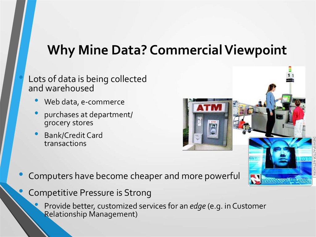
6. Why Mine Data? Commercial Viewpoint

Lots of data is being collected
and warehoused
Web data, e-commerce
purchases at department/
grocery stores
Bank/Credit Card
transactions
Computers have become cheaper and more powerful
Competitive Pressure is Strong
Provide better, customized services for an edge (e.g. in Customer
Relationship Management)

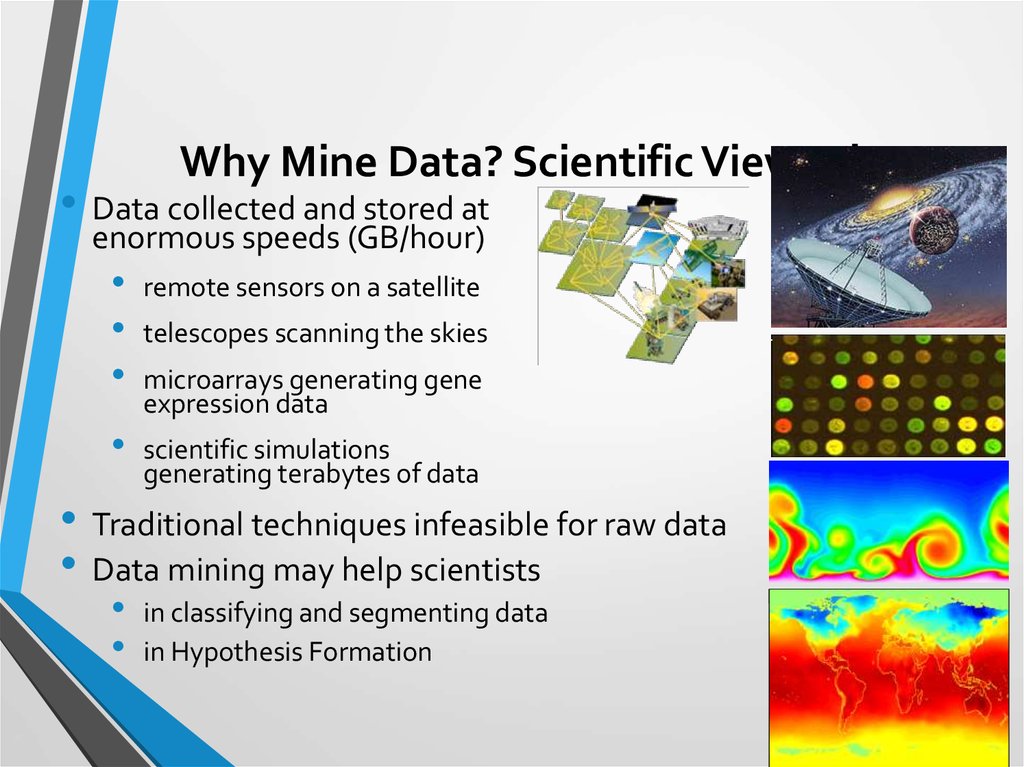
7. Why Mine Data? Scientific Viewpoint

• Data collected and stored at
enormous speeds (GB/hour)
remote sensors on a satellite
telescopes scanning the skies
microarrays generating gene
expression data
scientific simulations
generating terabytes of data
• Traditional techniques infeasible for raw data
• Data mining may help scientists
in classifying and segmenting data
in Hypothesis Formation

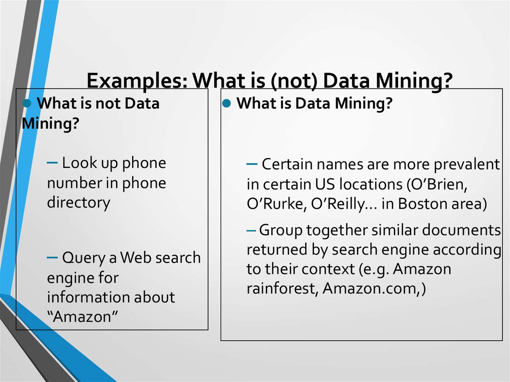
8. Examples: What is (not) Data Mining?

What is not Data
What is Data Mining?
Mining?
– Look up phone
– Certain names are more prevalent
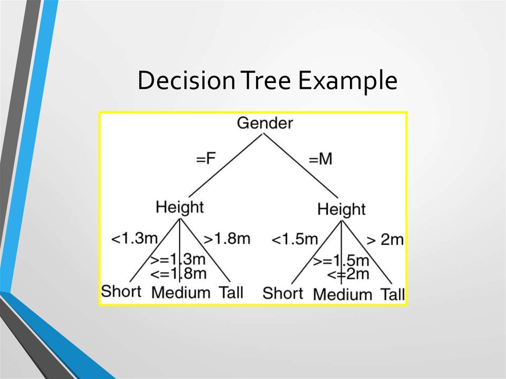
number in phone
directory
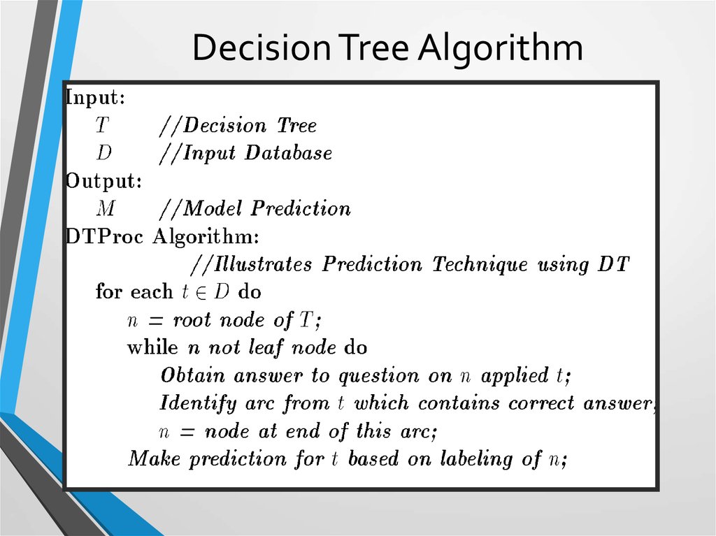
in certain US locations (O’Brien,
O’Rurke, O’Reilly… in Boston area)
– Query a Web search
– Group together similar documents
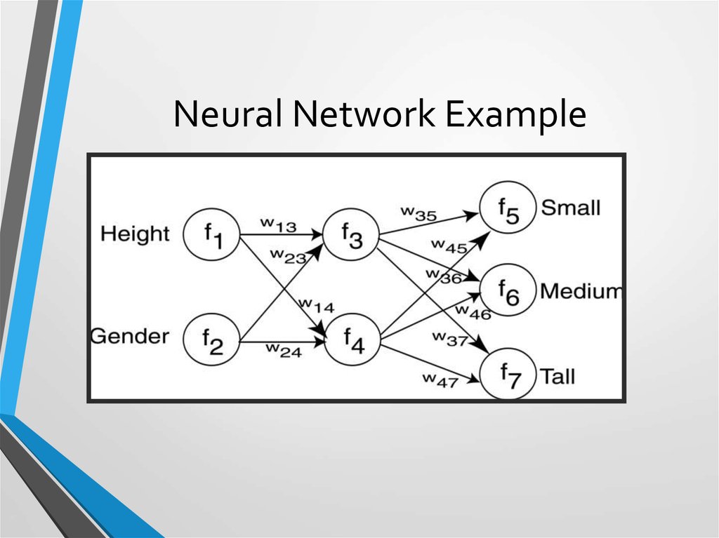
returned by search engine according
to their context (e.g. Amazon
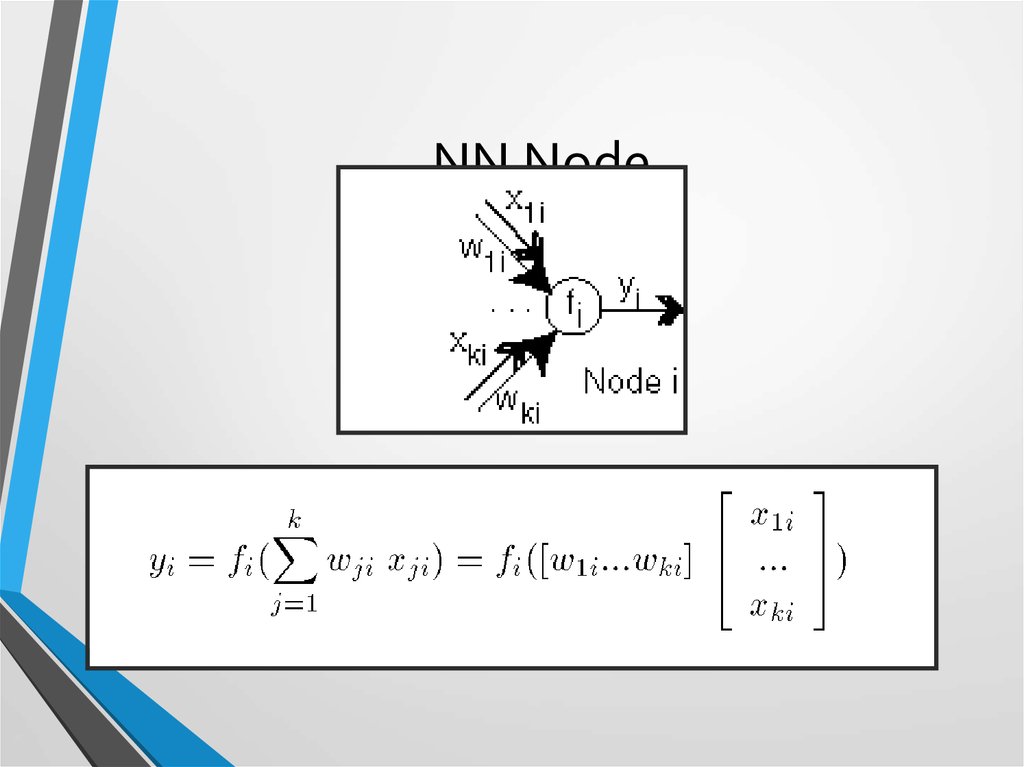
rainforest, Amazon.com,)
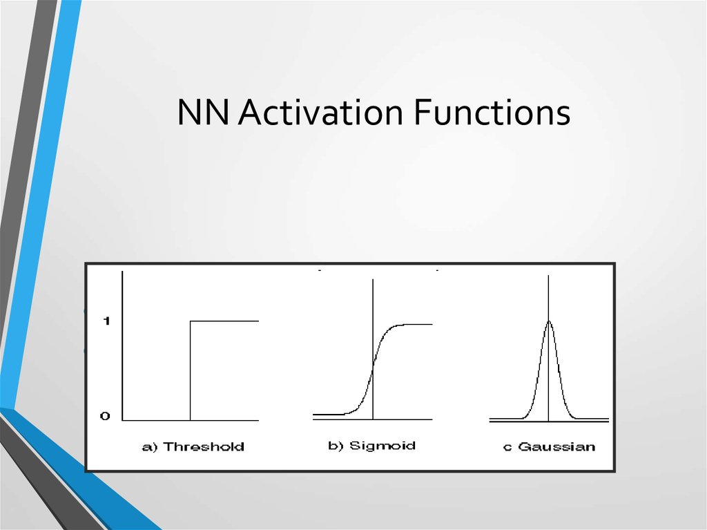
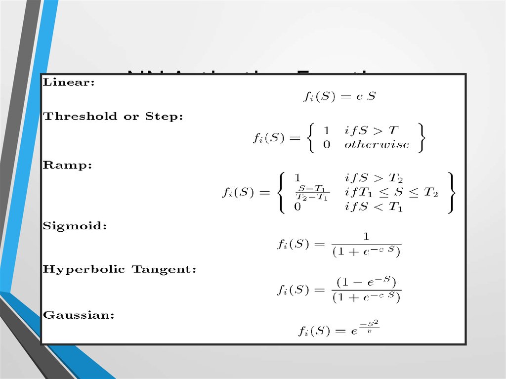
engine for
information about
“Amazon”

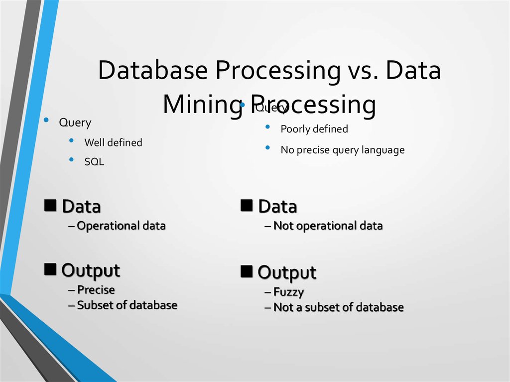
9. Database Processing vs. Data Mining Processing

Database Processing vs. Data
• Processing
Query
Mining
Query
Well defined
Poorly defined
No precise query language
SQL
Data
– Operational data
Output
– Precise
– Subset of database
Data
– Not operational data
Output
– Fuzzy
– Not a subset of database

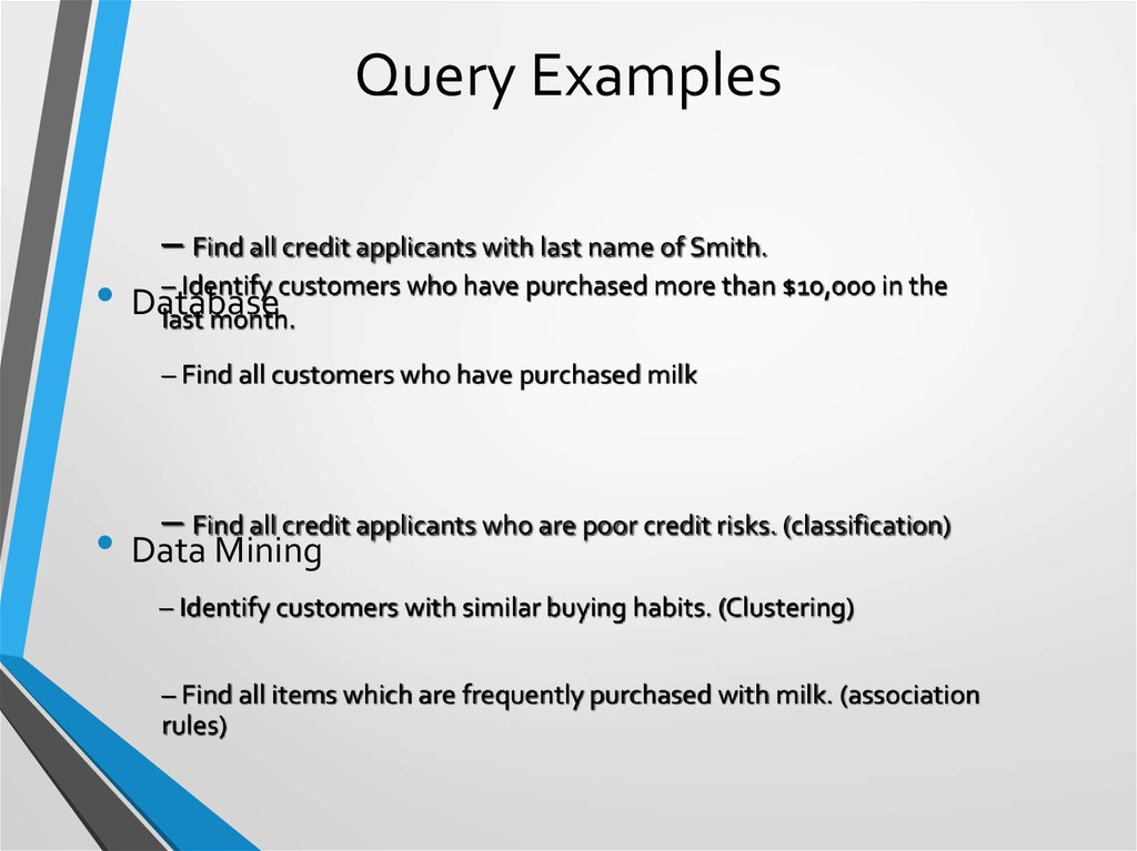
10. Query Examples

– Find all credit applicants with last name of Smith.
– Identify customers who have purchased more than $10,000 in the
• Database
last month.
– Find all customers who have purchased milk
– Find all credit applicants who are poor credit risks. (classification)
• Data Mining
– Identify customers with similar buying habits. (Clustering)
– Find all items which are frequently purchased with milk. (association
rules)

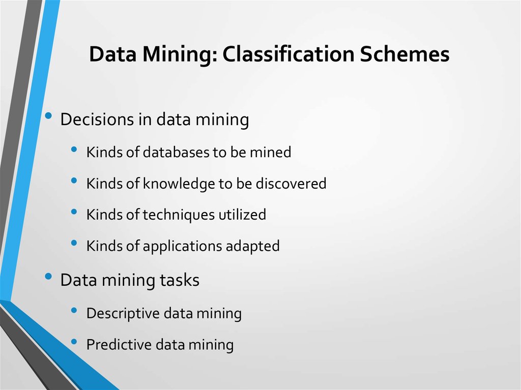
11. Data Mining: Classification Schemes

• Decisions in data mining
Kinds of databases to be mined
Kinds of knowledge to be discovered
Kinds of techniques utilized
Kinds of applications adapted
• Data mining tasks
Descriptive data mining
Predictive data mining

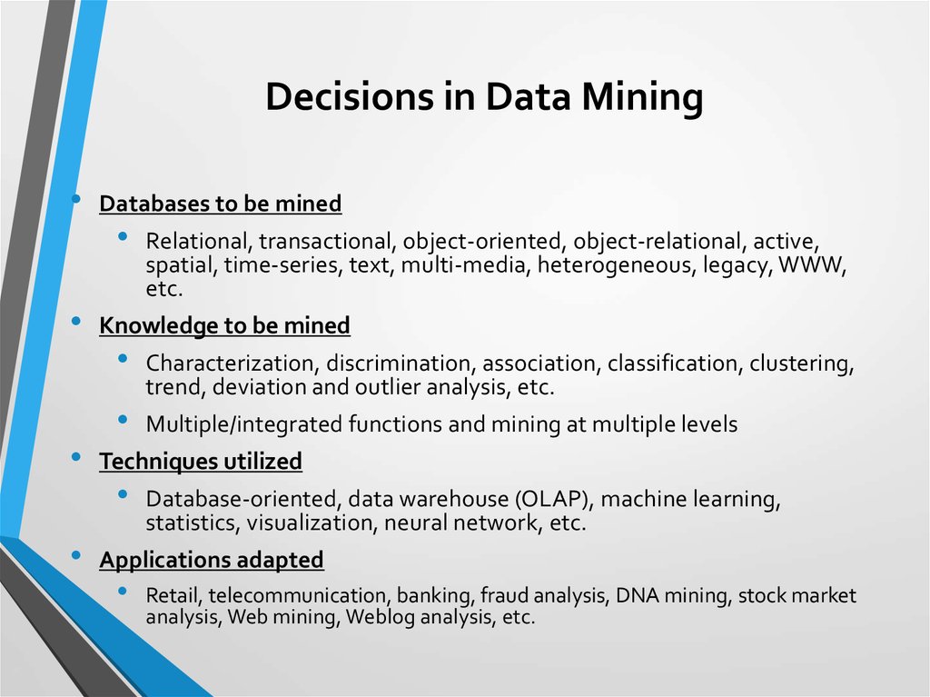
12. Decisions in Data Mining

Databases to be mined
Relational, transactional, object-oriented, object-relational, active,
spatial, time-series, text, multi-media, heterogeneous, legacy, WWW,
etc.
Knowledge to be mined
Characterization, discrimination, association, classification, clustering,
trend, deviation and outlier analysis, etc.
Multiple/integrated functions and mining at multiple levels
Techniques utilized
Database-oriented, data warehouse (OLAP), machine learning,
statistics, visualization, neural network, etc.
Applications adapted
Retail, telecommunication, banking, fraud analysis, DNA mining, stock market
analysis, Web mining, Weblog analysis, etc.

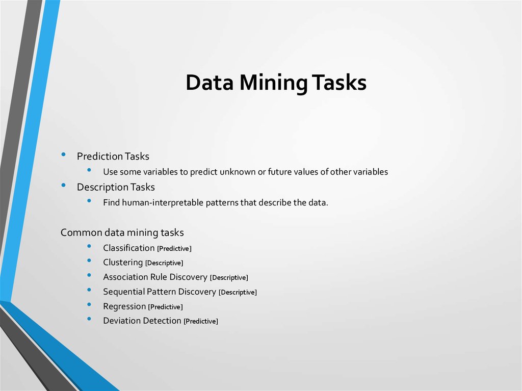
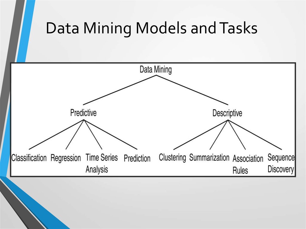
13. Data Mining Tasks

Prediction Tasks
Use some variables to predict unknown or future values of other variables
Description Tasks
Find human-interpretable patterns that describe the data.
Common data mining tasks
Classification [Predictive]
Clustering [Descriptive]
Association Rule Discovery [Descriptive]
Sequential Pattern Discovery [Descriptive]
Regression [Predictive]
Deviation Detection [Predictive]

14. Data Mining Models and Tasks

15. Classification

16. Classification: Definition

• Given a collection of records (training set )
Each record contains a set of attributes, one of the attributes is the
class.
• Find a model for class attribute as a function of the
values of other attributes.
• Goal: previously unseen records should be assigned a
class as accurately as possible.
A test set is used to determine the accuracy of the model. Usually,
the given data set is divided into training and test sets, with training
set used to build the model and test set used to validate it.

17. An Example

Classification
An Example
(from Pattern Classification by Duda & Hart & Stork –
Second Edition, 2001)
• A fish-packing plant wants to automate the
process of sorting incoming fish according to
species
• As a pilot project, it is decided to try to separate
sea bass from salmon using optical sensing

18. An Example (continued)

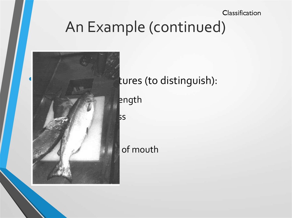
Classification
An Example (continued)
Features (to distinguish):
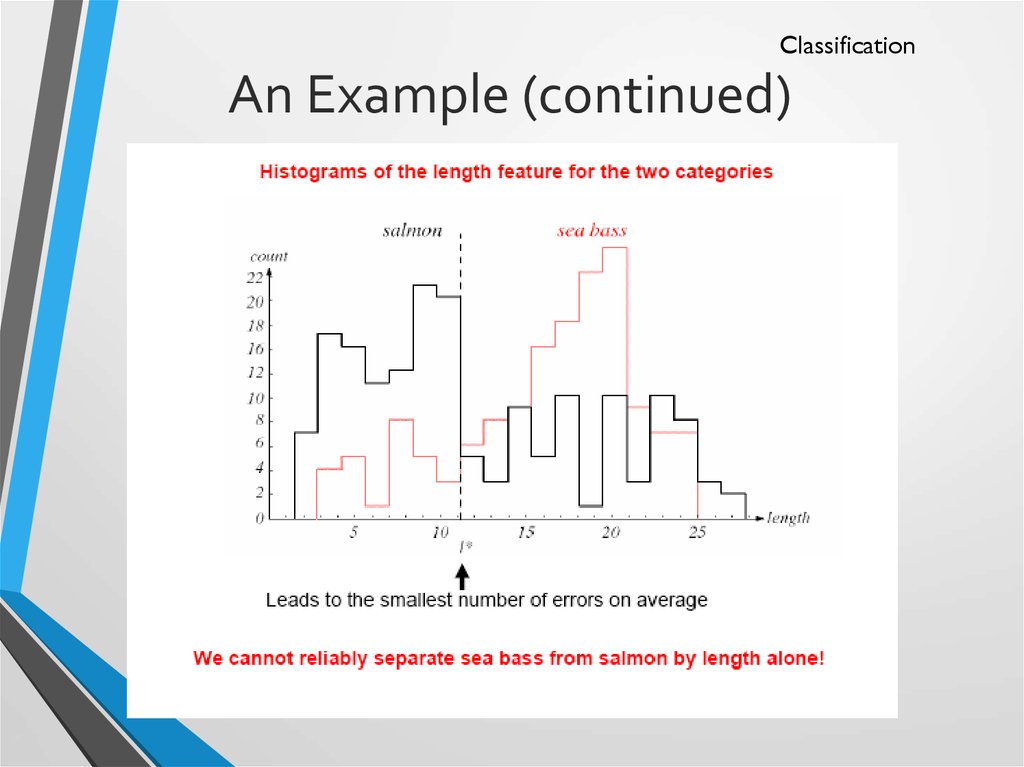
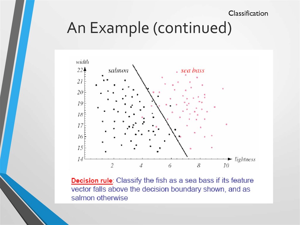
Length
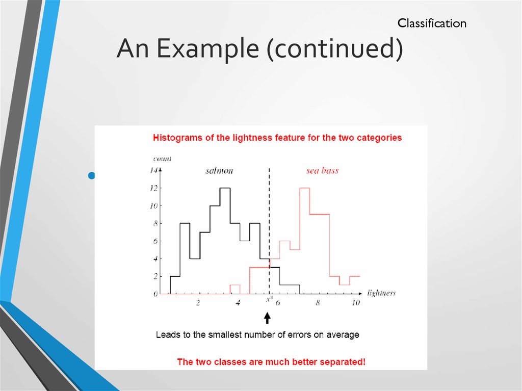
Lightness
Width
Position of mouth

19. An Example (continued)

Classification
An Example (continued)
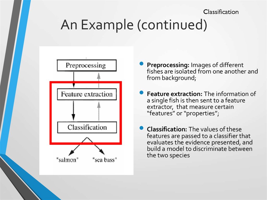
Preprocessing: Images of different
fishes are isolated from one another and
from background;
Feature extraction: The information of
a single fish is then sent to a feature
extractor, that measure certain
“features” or “properties”;
Classification: The values of these
features are passed to a classifier that
evaluates the evidence presented, and
build a model to discriminate between
the two species

20. An Example (continued)

Classification
An Example (continued)
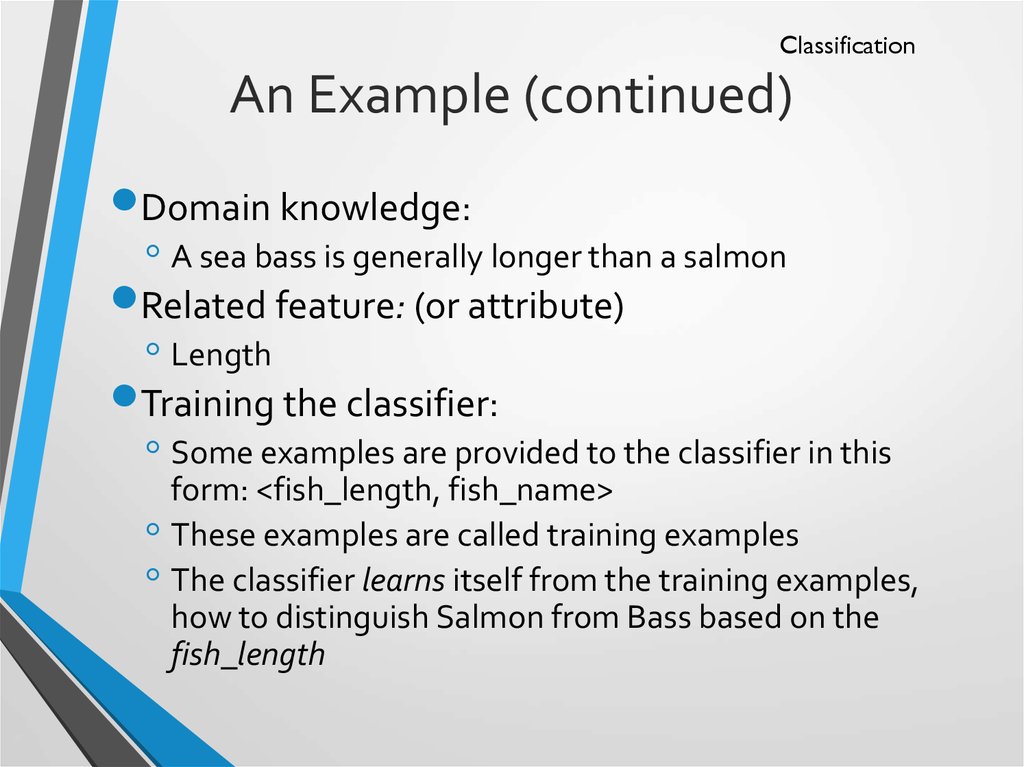
Domain knowledge:
◦ A sea bass is generally longer than a salmon
Related feature: (or attribute)
◦ Length
Training the classifier:
◦ Some examples are provided to the classifier in this
form: <fish_length, fish_name>
◦ These examples are called training examples
◦ The classifier learns itself from the training examples,
how to distinguish Salmon from Bass based on the
fish_length

21. An Example (continued)

Classification
An Example (continued)
Classification model (hypothesis):
◦ The classifier generates a model from the training
data to classify future examples (test examples)
◦ An example of the model is a rule like this:
◦ If Length >= l* then sea bass otherwise salmon
◦ Here the value of l* determined by the classifier
Testing the model
◦ Once we get a model out of the classifier, we may
use the classifier to test future examples
◦ The test data is provided in the form <fish_length>
◦ The classifier outputs <fish_type> by checking
fish_length against the model

22. An Example (continued)

Classification
An Example (continued)
Training
Data
Test/Unlabele
d Data
Preprocessing
, and feature
extraction
Preprocessing
, and feature
extraction
Feature vector
Feature vector
Training
Testing
against
model/
Classification
Model
Prediction/
Evaluation
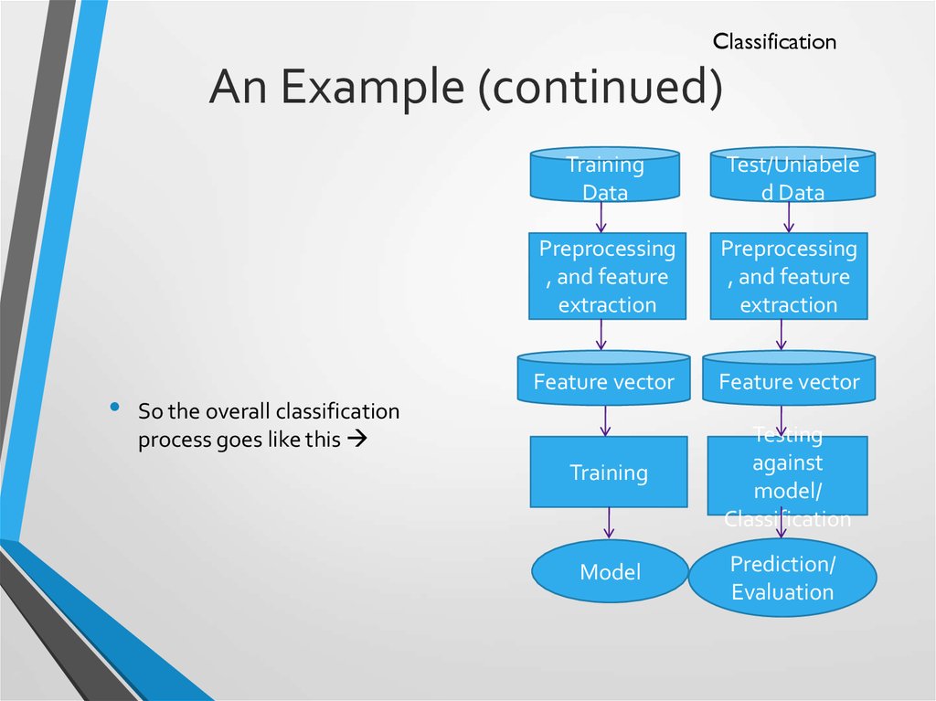
So the overall classification
process goes like this

23. An Example (continued)

Classification
An Example (continued)
Preprocessing,
Feature
extraction
Training data
12, salmon
15, sea bass
8, salmon
5, sea bass
Training
If len > 12,
then sea bass
else salmon
Model
Feature vector
Labeled data
Preprocessing,
Feature
extraction
Test data
Unlabeled data
15, salmon
10, salmon
18, ?
8, ?
Feature vector
Test/
Classify
sea bass (error!)
salmon (correct)
sea bass
salmon
Evaluation/Prediction

24. An Example (continued)

Classification
An Example (continued)
• Why error?
Insufficient training data
Too few features
Too many/irrelevant features
Overfitting / specialization

25. An Example (continued)

Classification
An Example (continued)

26. An Example (continued)

Classification
An Example (continued)
• New Feature:
• Average lightness of the fish scales

27. An Example (continued)

Classification
An Example (continued)

28. An Example (continued)

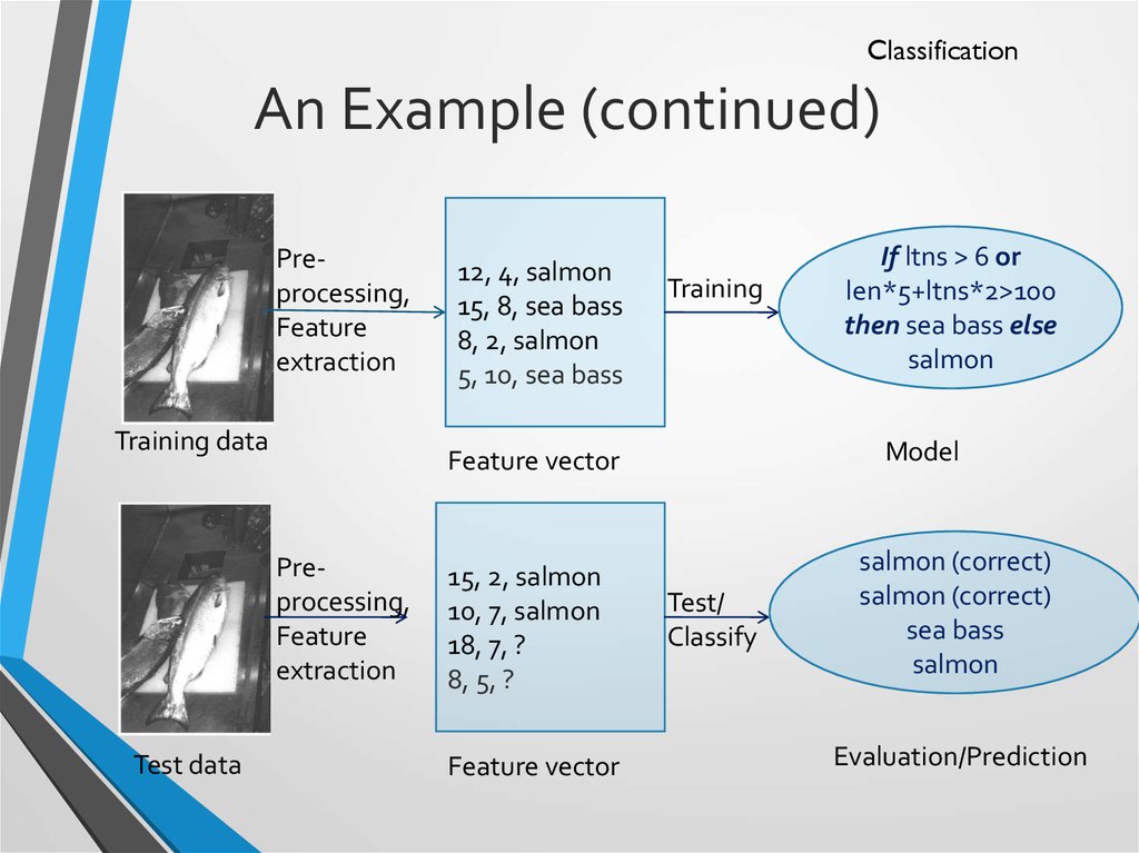
Classification
An Example (continued)
Preprocessing,
Feature
extraction
Training data
Training
15, 2, salmon
10, 7, salmon
18, 7, ?
8, 5, ?
Feature vector
If ltns > 6 or
len*5+ltns*2>100
then sea bass else
salmon
Model
Feature vector
Preprocessing,
Feature
extraction
Test data
12, 4, salmon
15, 8, sea bass
8, 2, salmon
5, 10, sea bass
Test/
Classify
salmon (correct)
salmon (correct)
sea bass
salmon
Evaluation/Prediction

29. Terms

Classification
Terms
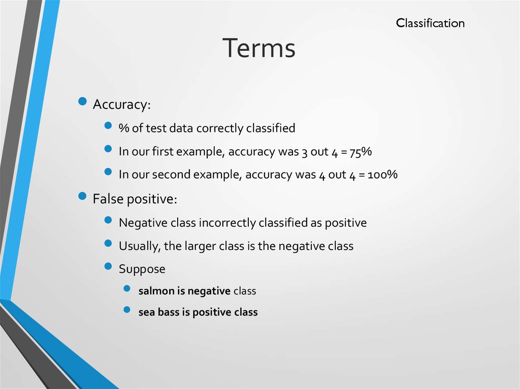
Accuracy:
% of test data correctly classified
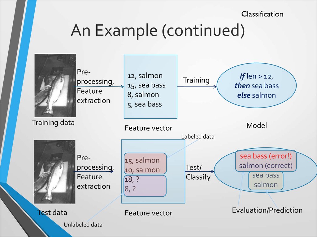
In our first example, accuracy was 3 out 4 = 75%
In our second example, accuracy was 4 out 4 = 100%
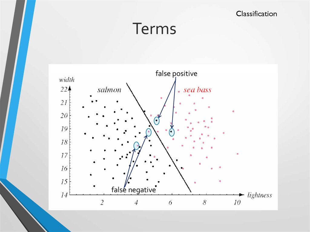
False positive:
Negative class incorrectly classified as positive
Usually, the larger class is the negative class
Suppose
salmon is negative class
sea bass is positive class

30. Terms

Classification
Terms
false positive
false negative

31. Terms

Classification
Terms
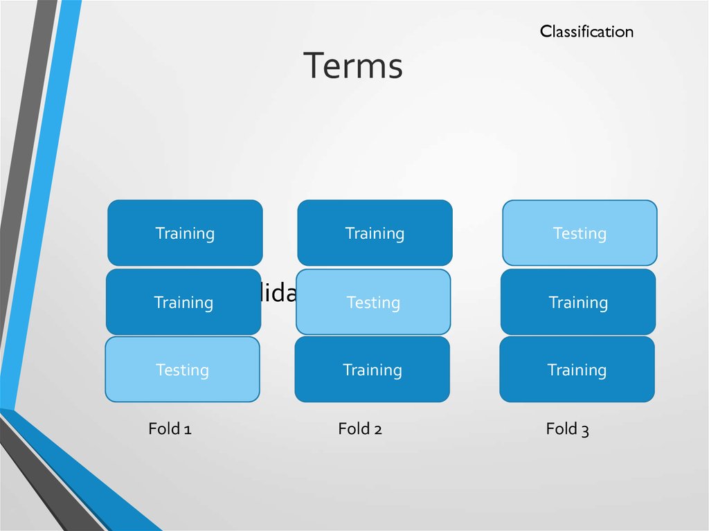
Training
Training
Training
Cross validation Testing
(3 fold)
Testing
Fold 1
Testing
Training
Training
Training
Fold 2
Fold 3

32. Classification Example 2

Tid Refund Marital
Status
Taxable
Income Cheat
Refund Marital
Status
Taxable
Income Cheat
1
Yes
Single
125K
No
No
Single
75K
?
2
No
Married
100K
No
Yes
Married
50K
?
3
No
Single
70K
No
No
Married
150K
?
4
Yes
Married
120K
No
Yes
Divorced 90K
?
5
No
Divorced 95K
Yes
No
Single
40K
?
6
No
Married
No
No
Married
80K
?
60K
10
7
Yes
Divorced 220K
No
8
No
Single
85K
Yes
9
No
Married
75K
No
10
10
No
Single
90K
Yes
Training
Set
Learn
Classifier
Test
Set
Model

33. Classification: Application 1

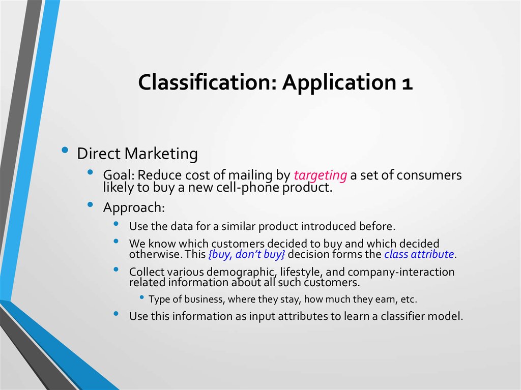
• Direct Marketing
Goal: Reduce cost of mailing by targeting a set of consumers
likely to buy a new cell-phone product.
Approach:
Use the data for a similar product introduced before.
We know which customers decided to buy and which decided
otherwise. This {buy, don’t buy} decision forms the class attribute.
Collect various demographic, lifestyle, and company-interaction
related information about all such customers.
• Type of business, where they stay, how much they earn, etc.
Use this information as input attributes to learn a classifier model.

34. Classification: Application 2

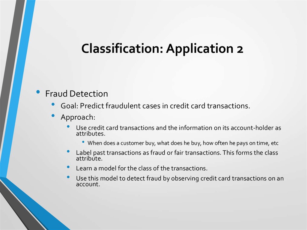
Fraud Detection
Goal: Predict fraudulent cases in credit card transactions.
Approach:
Use credit card transactions and the information on its account-holder as
attributes.
When does a customer buy, what does he buy, how often he pays on time, etc
Label past transactions as fraud or fair transactions. This forms the class
attribute.
Learn a model for the class of the transactions.
Use this model to detect fraud by observing credit card transactions on an
account.

35. Classification: Application 3

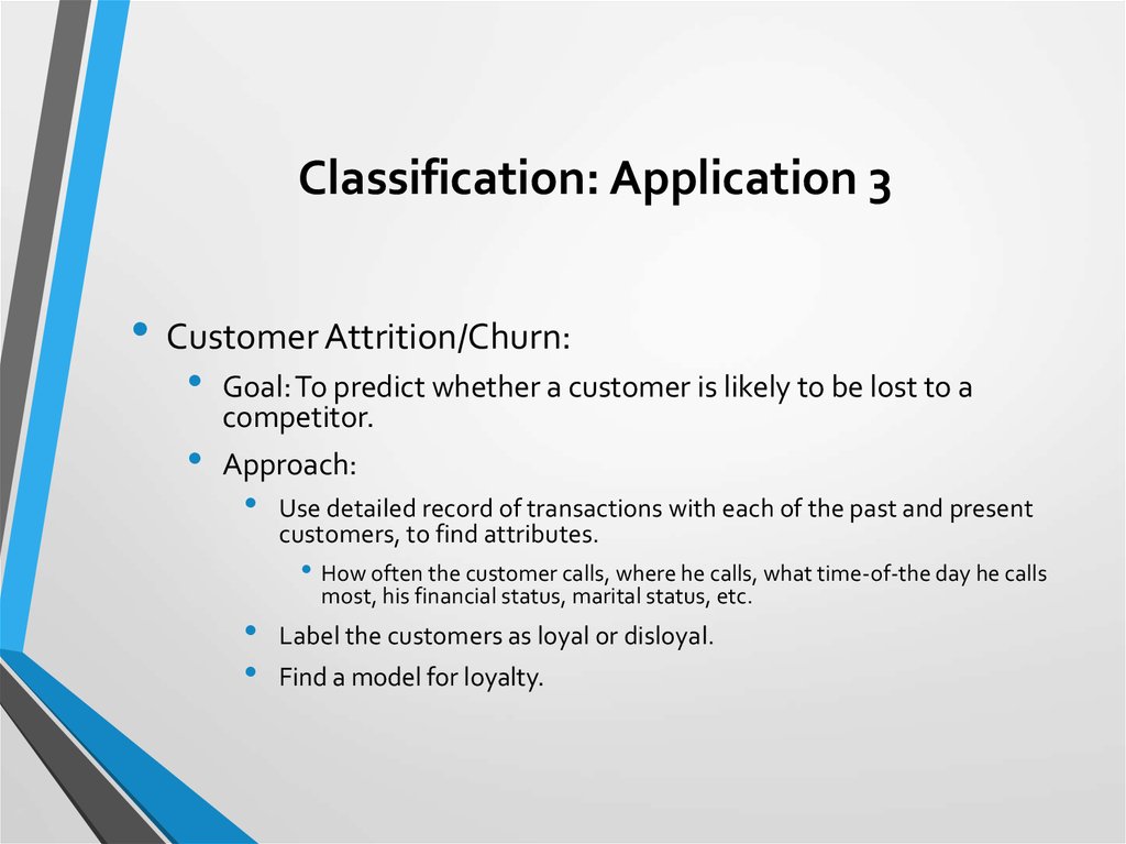
• Customer Attrition/Churn:
Goal: To predict whether a customer is likely to be lost to a
competitor.
Approach:
Use detailed record of transactions with each of the past and present
customers, to find attributes.
• How often the customer calls, where he calls, what time-of-the day he calls
most, his financial status, marital status, etc.
Label the customers as loyal or disloyal.
Find a model for loyalty.

36. Classification: Application 4

Sky Survey Cataloging
Goal: To predict class (star or galaxy) of sky objects, especially visually faint
ones, based on the telescopic survey images (from Palomar Observatory).
3000 images with 23,040 x 23,040 pixels per image.
Approach:
Segment the image.
Measure image attributes (features) - 40 of them per object.
Model the class based on these features.
Success Story: Could find 16 new high red-shift quasars, some of the farthest objects
that are difficult to find!

37. Classifying Galaxies

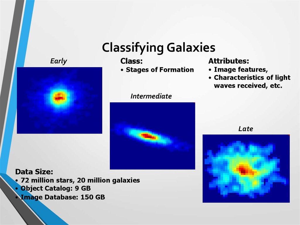
Early
Class:
• Stages of Formation
Attributes:
• Image features,
• Characteristics of light
waves received, etc.
Intermediate
Late
Data Size:
• 72 million stars, 20 million galaxies
• Object Catalog: 9 GB
• Image Database: 150 GB

38. Clustering

39. Clustering Definition

• Given a set of data points, each having a set of
attributes, and a similarity measure among them,
find clusters such that
• Data points in one cluster are more similar to one another.
• Data points in separate clusters are less similar to one
another.
• Similarity Measures:
• Euclidean Distance if attributes are continuous.
• Other Problem-specific Measures.

40. Illustrating Clustering

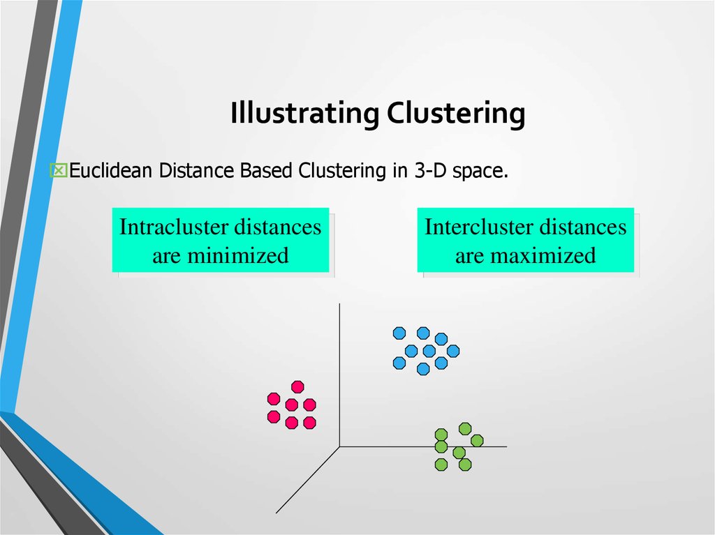
Euclidean Distance Based Clustering in 3-D space.
Intracluster distances
are minimized
Intercluster distances
are maximized

41. Clustering: Application 1

• Market Segmentation:
Goal: subdivide a market into distinct subsets of customers
where any subset may conceivably be selected as a market
target to be reached with a distinct marketing mix.
Approach:
Collect different attributes of customers based on their geographical
and lifestyle related information.
Find clusters of similar customers.
Measure the clustering quality by observing buying patterns of
customers in same cluster vs. those from different clusters.

42. Clustering: Application 2

• Document Clustering:
Goal: To find groups of documents that are similar to each
other based on the important terms appearing in them.
Approach: To identify frequently occurring terms in each
document. Form a similarity measure based on the
frequencies of different terms. Use it to cluster.
Gain: Information Retrieval can utilize the clusters to relate
a new document or search term to clustered documents.

43. Association rule mining

44. Association Rule Discovery: Definition

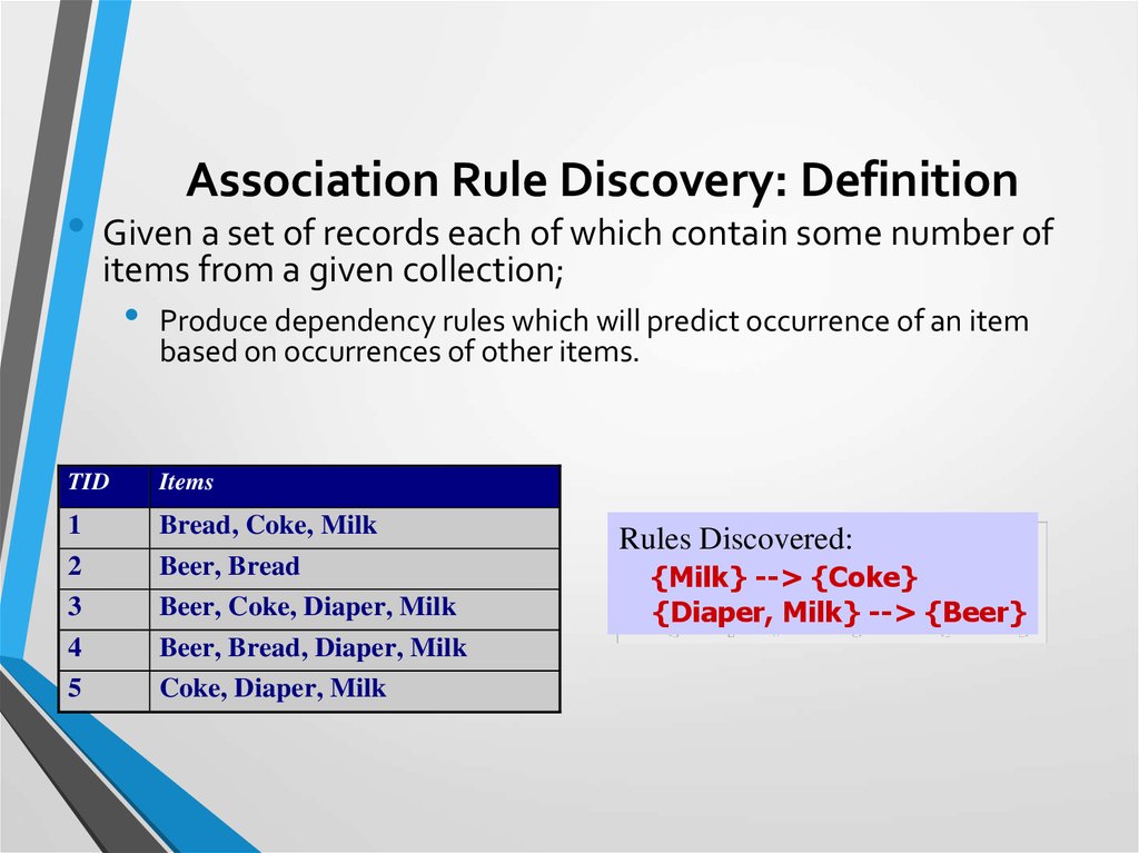
• Given a set of records each of which contain some number of
items from a given collection;
Produce dependency rules which will predict occurrence of an item
based on occurrences of other items.
TID
Items
1
2
Bread, Coke, Milk
Beer, Bread
3
Beer, Coke, Diaper, Milk
4
Beer, Bread, Diaper, Milk
5
Coke, Diaper, Milk
Rules Discovered:
{Milk} --> {Coke}
{Diaper, Milk} --> {Beer}

45. Association Rule Discovery: Application 1

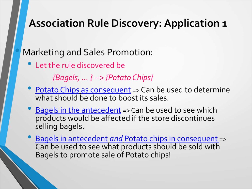
• Marketing and Sales Promotion:
• Let the rule discovered be
{Bagels, … } --> {Potato Chips}
Potato Chips as consequent => Can be used to determine
what should be done to boost its sales.
Bagels in the antecedent => Can be used to see which
products would be affected if the store discontinues
selling bagels.
Bagels in antecedent and Potato chips in consequent =>
Can be used to see what products should be sold with
Bagels to promote sale of Potato chips!

46. Association Rule Discovery: Application 2

• Supermarket shelf management.
• Goal: To identify items that are bought together by
sufficiently many customers.
• Approach: Process the point-of-sale data collected with
barcode scanners to find dependencies among items.
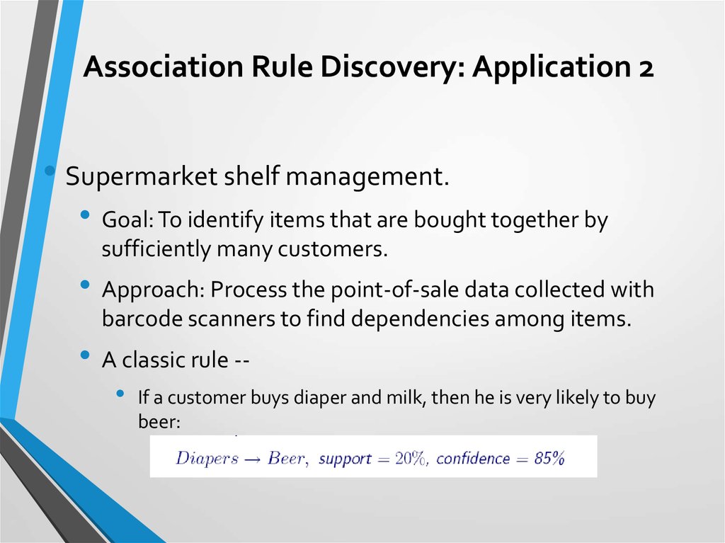
• A classic rule -
If a customer buys diaper and milk, then he is very likely to buy
beer:

47. SOME Classification techniques

48. Bayes Theorem

Posterior Probability: P(h1|xi)
Prior Probability: P(h1)
Bayes Theorem:
Assign probabilities of hypotheses given a data value.

49. Bayes Theorem Example

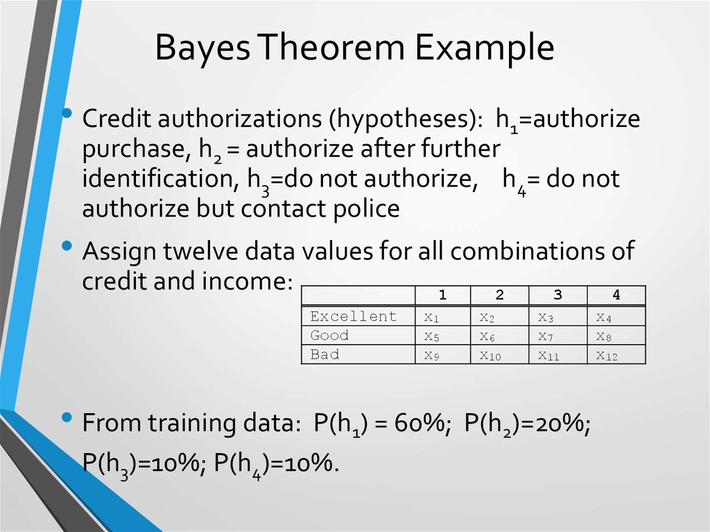
• Credit authorizations (hypotheses): h1=authorize
purchase, h2 = authorize after further
identification, h3=do not authorize, h4= do not
authorize but contact police
• Assign twelve data values for all combinations of
credit and income:
1
Excellent
Good
Bad
x1
x5
x9
2
3
4
x2
x6
x10
x3
x7
x11
x4
x8
x12
• From training data: P(h1) = 60%; P(h2)=20%;
P(h3)=10%; P(h4)=10%.

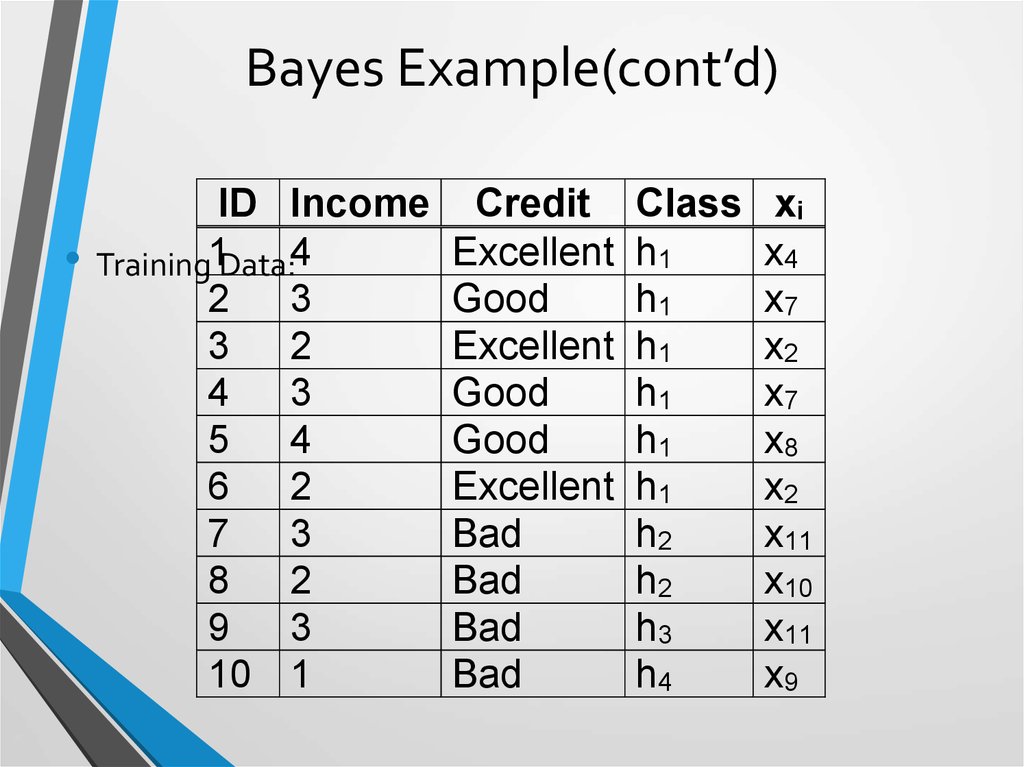
50. Bayes Example(cont’d)

ID Income
Training1Data:4
2
3
3
2
4
3
5
4
6
2
7
3
8
2
9
3
10 1
Credit
Excellent
Good
Excellent
Good
Good
Excellent
Bad
Bad
Bad
Bad
Class
h1
h1
h1
h1
h1
h1
h2
h2
h3
h4
xi
x4
x7
x2
x7
x8
x2
x11
x10
x11
x9

51. Bayes Example(cont’d)

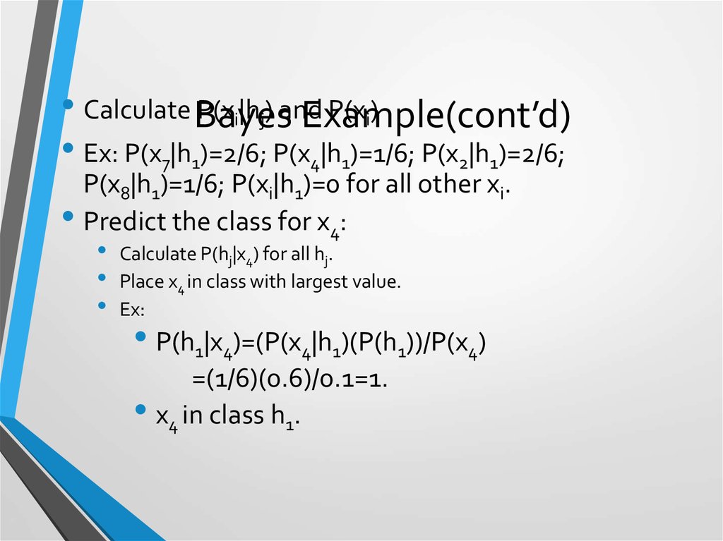
• Calculate Bayes
P(xi|hj) and
P(xi)
Example(cont’d)
• Ex: P(x7|h1)=2/6; P(x4|h1)=1/6; P(x2|h1)=2/6;
P(x8|h1)=1/6; P(xi|h1)=0 for all other xi.
• Predict the class for x4:
• Calculate P(hj|x4) for all hj.
• Place x4 in class with largest value.
• Ex:
• P(h1|x4)=(P(x4|h1)(P(h1))/P(x4)
=(1/6)(0.6)/0.1=1.
• x4 in class h1.

52. Hypothesis Testing

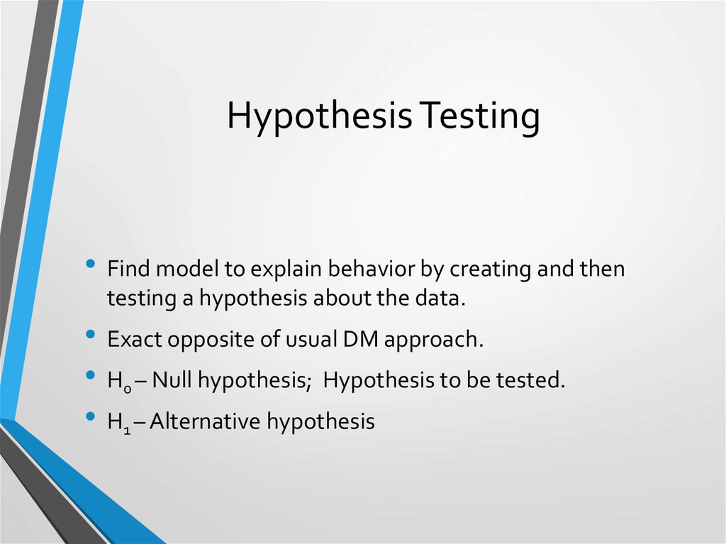
• Find model to explain behavior by creating and then
testing a hypothesis about the data.
• Exact opposite of usual DM approach.
• H0 – Null hypothesis; Hypothesis to be tested.
• H1 – Alternative hypothesis

53. Chi Squared Statistic

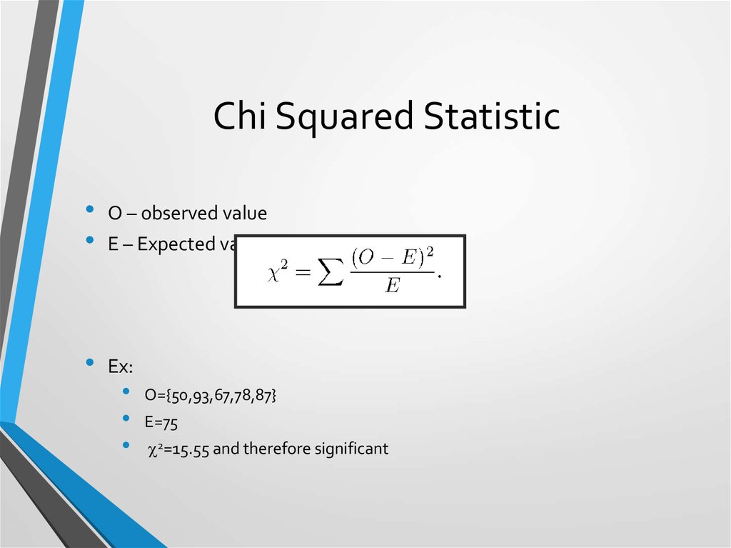
O – observed value
E – Expected value based on hypothesis.
Ex:
O={50,93,67,78,87}
E=75
c2=15.55 and therefore significant

54. Regression

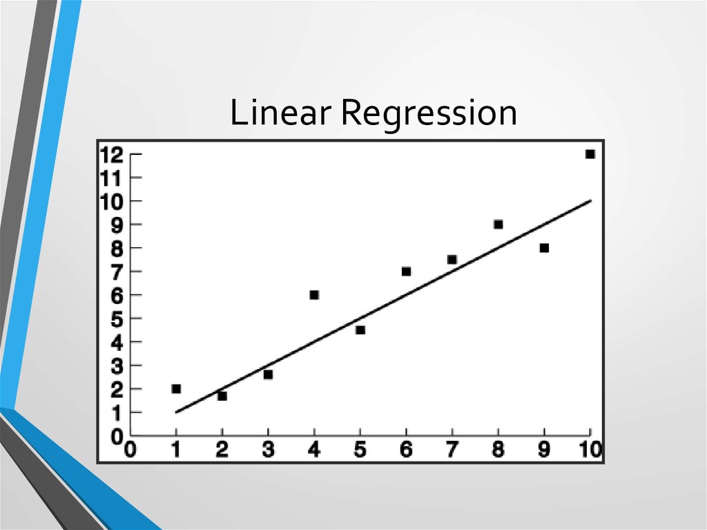
• Predict future values based on past values
• Linear Regression assumes linear relationship exists.
y = c0 + c1 x1 + … + cn xn
• Find values to best fit the data

55. Linear Regression

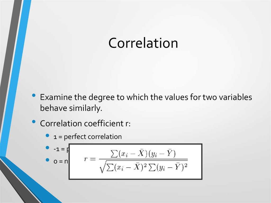
56. Correlation

• Examine the degree to which the values for two variables
behave similarly.
• Correlation coefficient r:
1 = perfect correlation
-1 = perfect but opposite correlation
0 = no correlation

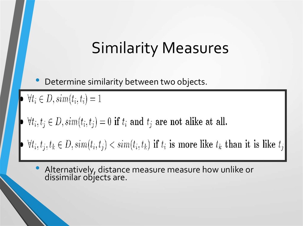
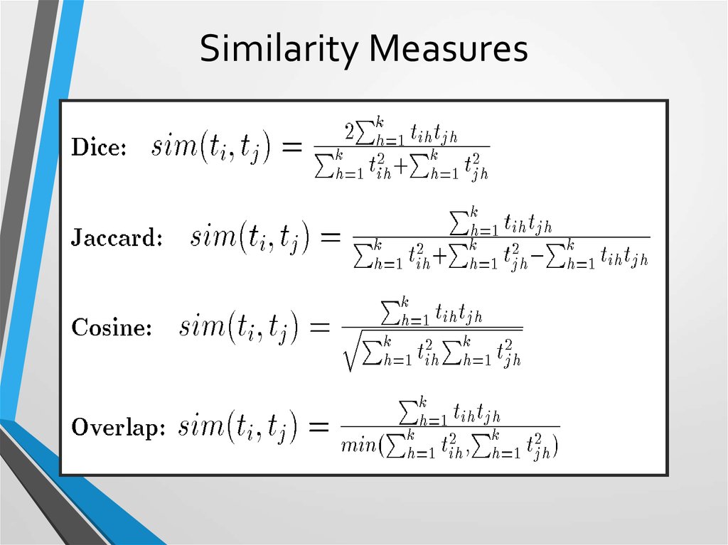
57. Similarity Measures

Determine similarity between two objects.
Similarity characteristics:
Alternatively, distance measure measure how unlike or
dissimilar objects are.

58. Similarity Measures

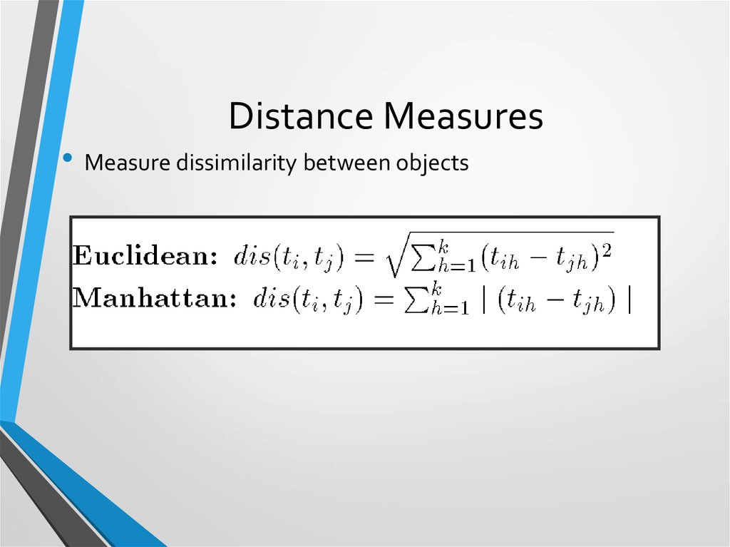
59. Distance Measures

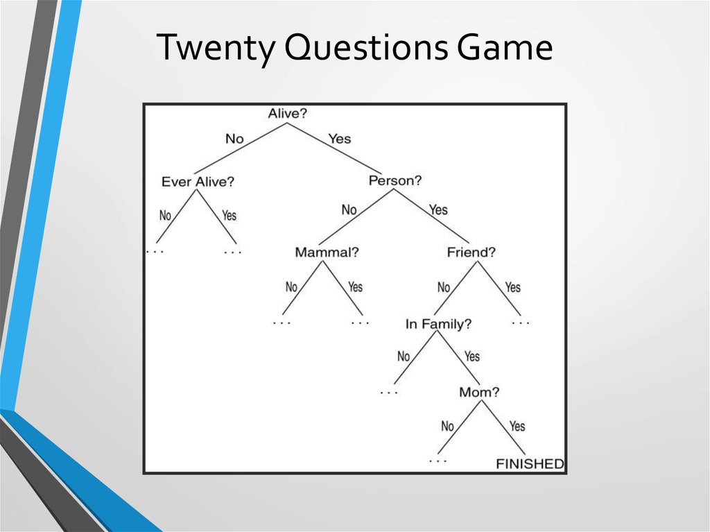
• Measure dissimilarity between objects

60. Twenty Questions Game

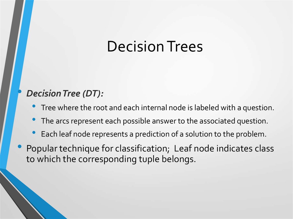
61. Decision Trees

• Decision Tree (DT):
Tree where the root and each internal node is labeled with a question.
The arcs represent each possible answer to the associated question.
Each leaf node represents a prediction of a solution to the problem.
• Popular technique for classification; Leaf node indicates class
to which the corresponding tuple belongs.

62. Decision Tree Example

63. Decision Trees

• A Decision Tree Model is a computational model
consisting of three parts:
• Decision Tree
• Algorithm to create the tree
• Algorithm that applies the tree to data
• Creation of the tree is the most difficult part.
• Processing is basically a search similar to that in a
binary search tree (although DT may not be
binary).

64. Decision Tree Algorithm

65. DT Advantages/Disadvantages

• Advantages:
Easy to understand.
Easy to generate rules
• Disadvantages:
May suffer from overfitting.
Classifies by rectangular partitioning.
Does not easily handle nonnumeric data.
Can be quite large – pruning is necessary.

66. Neural Networks

• Based on observed functioning of human brain.
• (Artificial Neural Networks (ANN)
• Our view of neural networks is very simplistic.
• We view a neural network (NN) from a graphical viewpoint.
• Alternatively, a NN may be viewed from the perspective of
matrices.
Used in pattern recognition, speech recognition, computer
vision, and classification.

67. Neural Networks

• Neural Network (NN) is a directed graph F=<V,A>
with vertices V={1,2,…,n} and arcs
A={<i,j>|1<=i,j<=n}, with the following restrictions:
• V is partitioned into a set of input nodes, VI, hidden nodes, VH,
and output nodes, VO.
The vertices are also partitioned into layers
Any arc <i,j> must have node i in layer h-1 and node j in layer h.
Arc <i,j> is labeled with a numeric value wij.
Node i is labeled with a function fi.

68. Neural Network Example

69. NN Node

70. NN Activation Functions

• Functions associated with nodes in graph.
• Output may be in range [-1,1] or [0,1]

71. NN Activation Functions

72. NN Learning

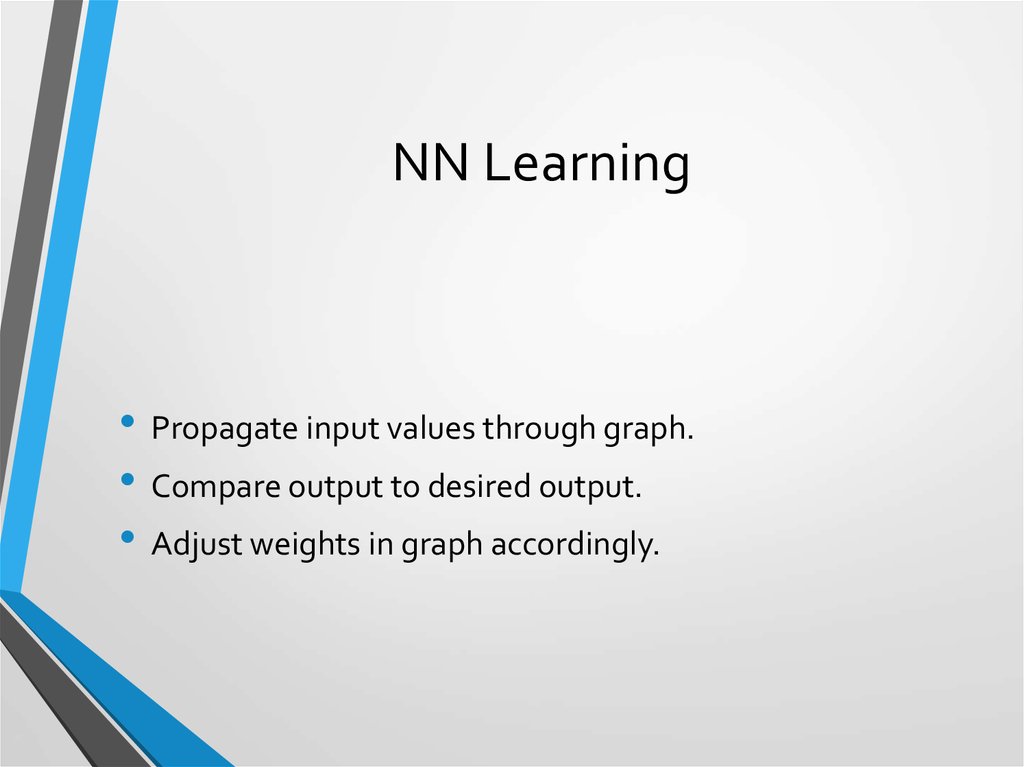
• Propagate input values through graph.
• Compare output to desired output.
• Adjust weights in graph accordingly.

73. Neural Networks

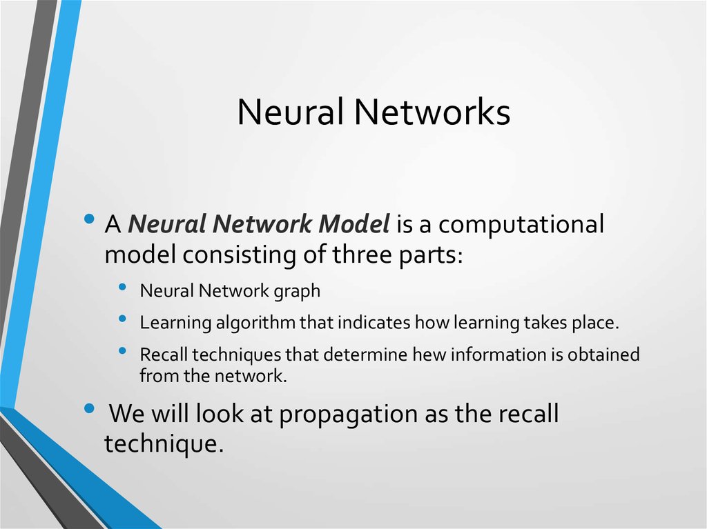
• A Neural Network Model is a computational
model consisting of three parts:
• Neural Network graph
• Learning algorithm that indicates how learning takes place.
• Recall techniques that determine hew information is obtained
from the network.
We will look at propagation as the recall
technique.

74. NN Advantages

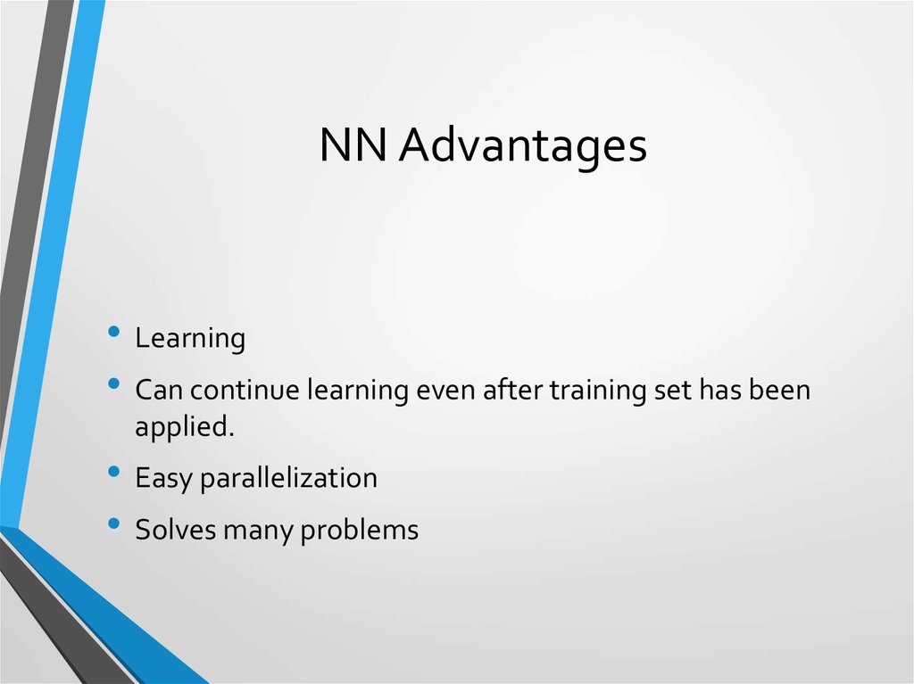
• Learning
• Can continue learning even after training set has been
applied.
• Easy parallelization
• Solves many problems

75. NN Disadvantages

• Difficult to understand
• May suffer from overfitting
• Structure of graph must be determined a priori.
• Input values must be numeric.
• Verification difficult.