Game-Theoretic Methods in Machine Learning

1.

Game-Theoretic Methods in
Machine Learning
Marcello Pelillo
European Centre for Living Technology
Ca’ Foscari University, Venice
2nd Winter School on Data Analytics, Nizhny Novgorod, Russia, October 3-4, 2017

2.

From Cliques to Equilibria
Dominant-Set Clustering and Its Applications

3.

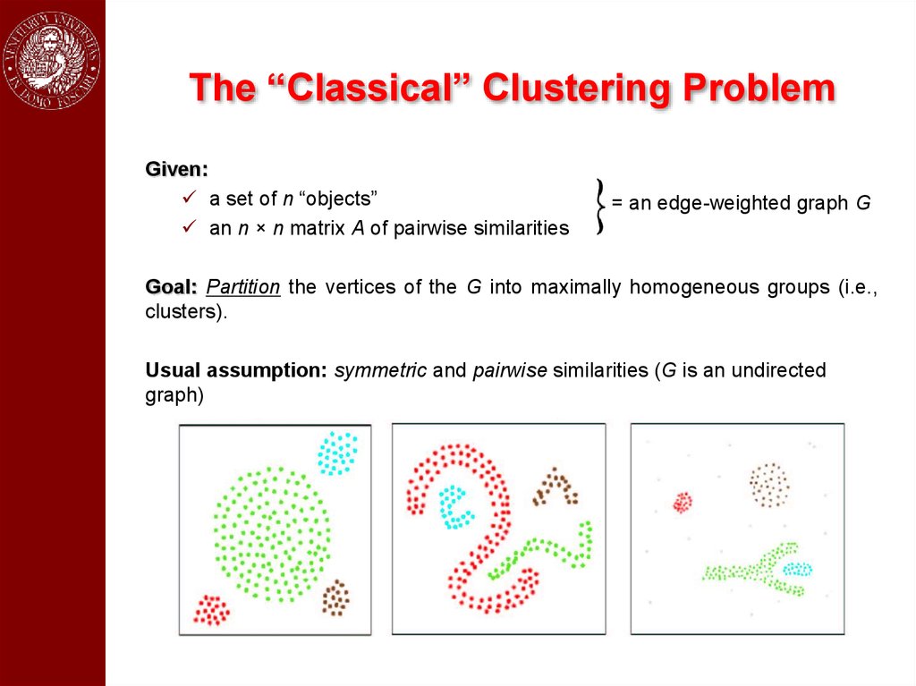
The “Classical” Clustering Problem
Given:
a set of n “objects”
an n × n matrix A of pairwise similarities
= an edge-weighted graph G
Goal: Partition the vertices of the G into maximally homogeneous groups (i.e.,
clusters).
Usual assumption: symmetric and pairwise similarities (G is an undirected
graph)

4.

Applications
Clustering problems abound in many areas of computer science and
engineering.
A short list of applications domains:
Image processing and computer vision
Computational biology and bioinformatics
Information retrieval
Document analysis
Medical image analysis
Data mining
Signal processing
…
For a review see, e.g., A. K. Jain, "Data clustering: 50 years beyond K-means,”
Pattern Recognition Letters 31(8):651-666, 2010.

5.

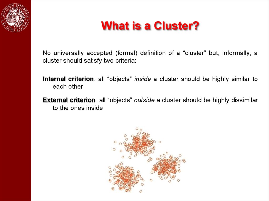
What is a Cluster?
No universally accepted (formal) definition of a “cluster” but, informally, a
cluster should satisfy two criteria:
Internal criterion: all “objects” inside a cluster should be highly similar to
each other
External criterion: all “objects” outside a cluster should be highly dissimilar
to the ones inside

6.

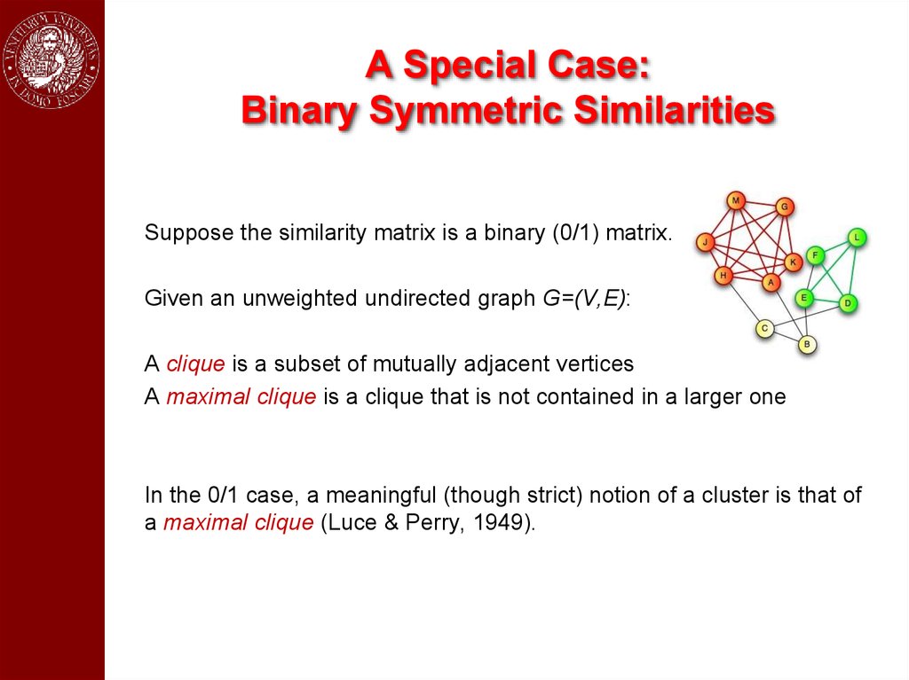
A Special Case:
Binary Symmetric Similarities
Suppose the similarity matrix is a binary (0/1) matrix.
Given an unweighted undirected graph G=(V,E):
A clique is a subset of mutually adjacent vertices
A maximal clique is a clique that is not contained in a larger one
In the 0/1 case, a meaningful (though strict) notion of a cluster is that of
a maximal clique (Luce & Perry, 1949).

7.

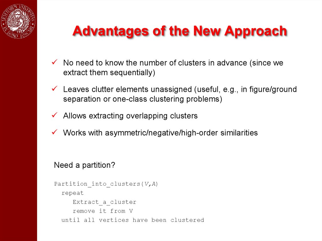
Advantages of the New Approach
No need to know the number of clusters in advance (since we
extract them sequentially)
Leaves clutter elements unassigned (useful, e.g., in figure/ground
separation or one-class clustering problems)
Allows extracting overlapping clusters
Works with asymmetric/negative/high-order similarities
Need a partition?
Partition_into_clusters(V,A)
repeat
Extract_a_cluster
remove it from V
until all vertices have been clustered

8.

What is Game Theory?
“The central problem of game theory was posed by von
Neumann as early as 1926 in Göttingen. It is the following:
If n players, P1,…, Pn, play a given game Γ, how must the ith
player, Pi, play to achieve the most favorable result for
himself?”
Harold W. Kuhn
Lectures on the Theory of Games (1953)
A few cornerstones in game theory
1921−1928: Emile Borel and John von Neumann give the first modern formulation of a
mixed strategy along with the idea of finding minimax solutions of normal-form
games.
1944, 1947: John von Neumann and Oskar Morgenstern publish Theory of Games and
Economic Behavior.
1950−1953: In four papers John Nash made seminal contributions to both noncooperative game theory and to bargaining theory.
1972−1982: John Maynard Smith applies game theory to biological problems thereby
founding “evolutionary game theory.”
late 1990’s −: Development of algorithmic game theory…

9.

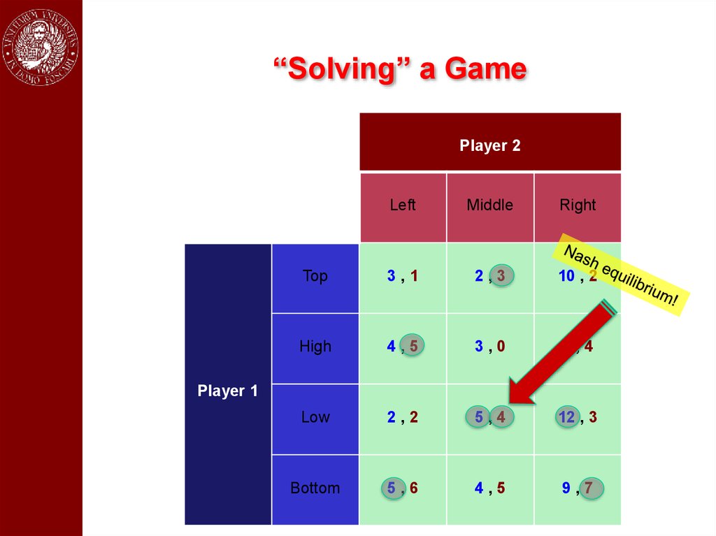
“Solving” a Game
Player 2
Left
Middle
Right
Top
3,1
2,3
10 , 2
High
4,5
3,0
6,4
Low
2,2
5,4
12 , 3
Bottom
5,6
4,5
9,7
Player 1

10.

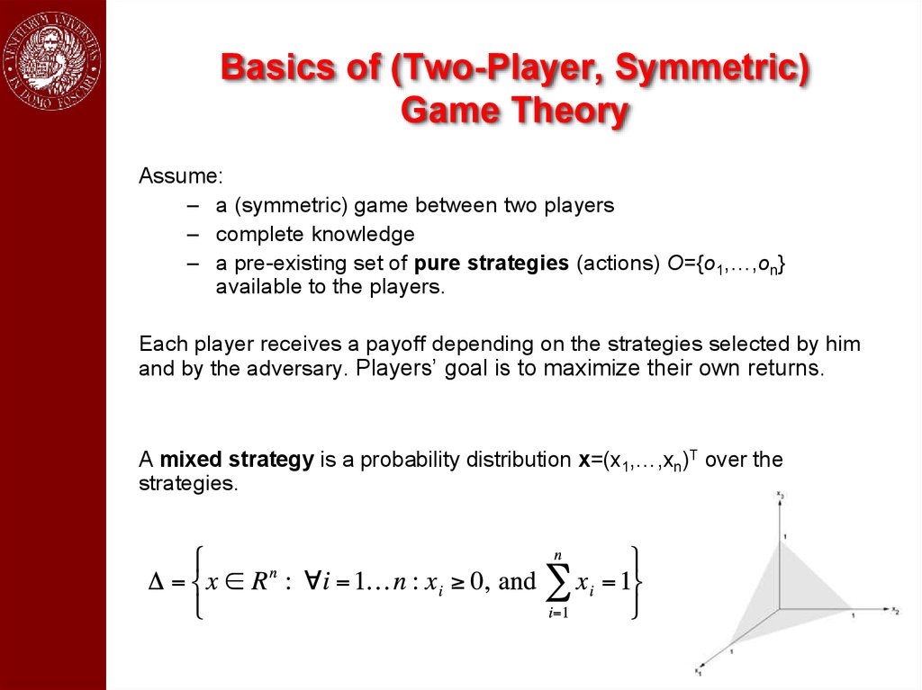
Basics of (Two-Player, Symmetric)
Game Theory
Assume:
– a (symmetric) game between two players
– complete knowledge
– a pre-existing set of pure strategies (actions) O={o1,…,on}
available to the players.
Each player receives a payoff depending on the strategies selected by him
and by the adversary. Players’ goal is to maximize their own returns.
A mixed strategy is a probability distribution x=(x1,…,xn)T over the
strategies.

11.

Nash Equilibria
Let A be an arbitrary payoff matrix: aij is the payoff obtained by playing i
while the opponent plays j.
The average payoff obtained by playing mixed strategy y while the
opponent plays x, is:
A mixed strategy x is a (symmetric) Nash equilibrium if
for all strategies y. (Best reply to itself.)
Theorem (Nash, 1951). Every finite normal-form game admits a mixedstrategy Nash equilibrium.

12.

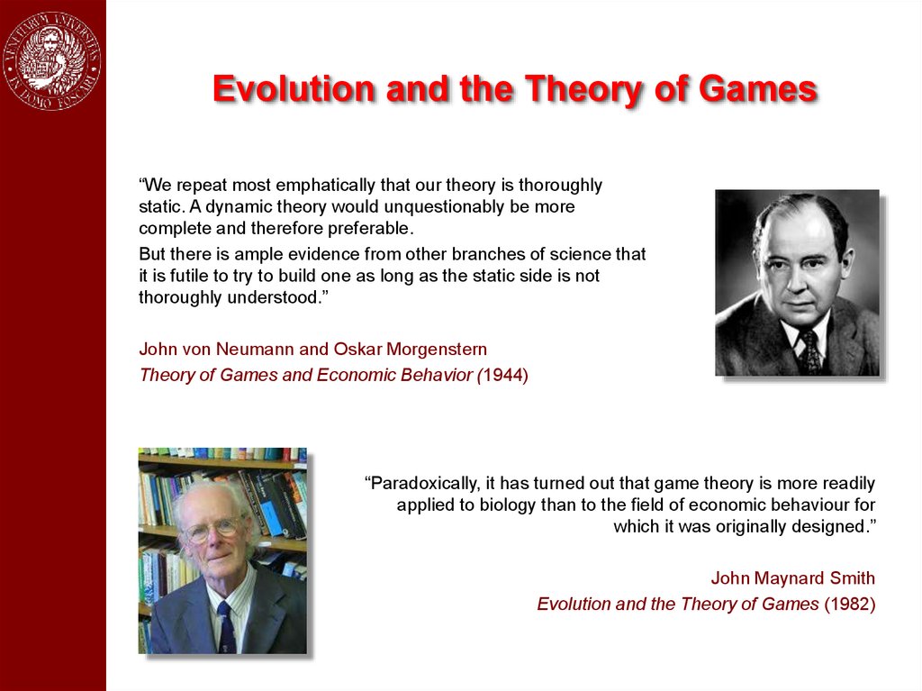
Evolution and the Theory of Games
“We repeat most emphatically that our theory is thoroughly
static. A dynamic theory would unquestionably be more
complete and therefore preferable.
But there is ample evidence from other branches of science that
it is futile to try to build one as long as the static side is not
thoroughly understood.”
John von Neumann and Oskar Morgenstern
Theory of Games and Economic Behavior (1944)
“Paradoxically, it has turned out that game theory is more readily
applied to biology than to the field of economic behaviour for
which it was originally designed.”
John Maynard Smith
Evolution and the Theory of Games (1982)

13.

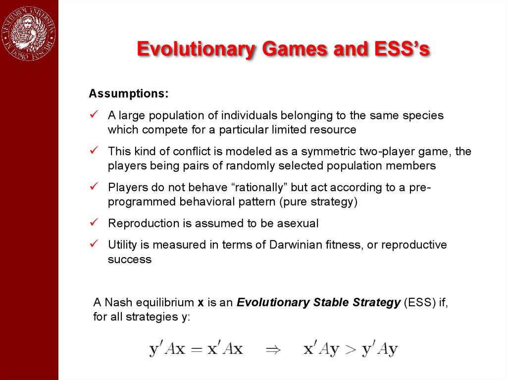
Evolutionary Games and ESS’s
Assumptions:
A large population of individuals belonging to the same species
which compete for a particular limited resource
This kind of conflict is modeled as a symmetric two-player game, the
players being pairs of randomly selected population members
Players do not behave “rationally” but act according to a preprogrammed behavioral pattern (pure strategy)
Reproduction is assumed to be asexual
Utility is measured in terms of Darwinian fitness, or reproductive
success
A Nash equilibrium x is an Evolutionary Stable Strategy (ESS) if,
for all strategies y:

14.

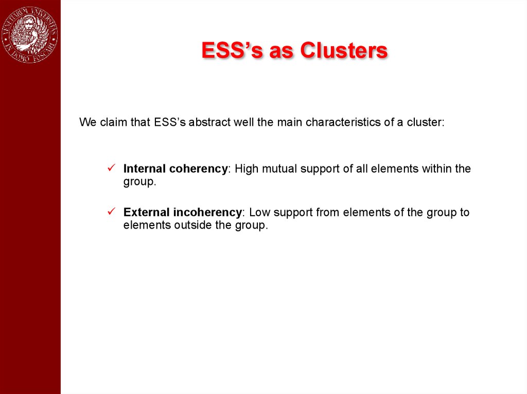
ESS’s as Clusters
We claim that ESS’s abstract well the main characteristics of a cluster:
Internal coherency: High mutual support of all elements within the
group.
External incoherency: Low support from elements of the group to
elements outside the group.

15.

Basic Definitions
Let S ⊆ V be a non-empty subset of vertices, and i∈S.
The (average) weighted degree of i w.r.t. S is defined as:
awdegS(i) =
1
aij
å
| S| j ÎS
Moreover, if j ∉ S, we define:
i
fS(i, j) = aij - awdegS(i)
S
Intuitively, φS(i,j) measures the similarity between vertices j and i, with
respect to the (average) similarity between vertex i and its neighbors in S.
j

16.

Assigning Weights to Vertices
Let S ⊆ V be a non-empty subset of vertices, and i∈S.
The weight of i w.r.t. S is defined as:
S-{i}
Further, the total weight of S is defined as:
j
W(S) = å wS(i)
i ÎS
i
S

17.

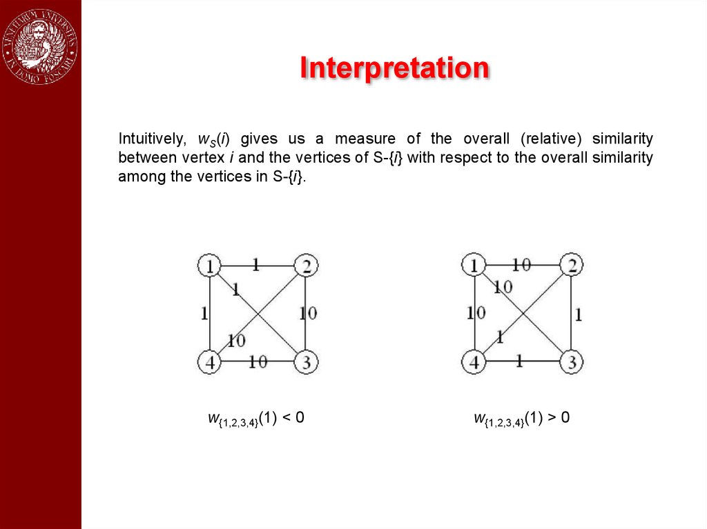
Interpretation
Intuitively, wS(i) gives us a measure of the overall (relative) similarity
between vertex i and the vertices of S-{i} with respect to the overall similarity
among the vertices in S-{i}.
w{1,2,3,4}(1) < 0
w{1,2,3,4}(1) > 0

18.

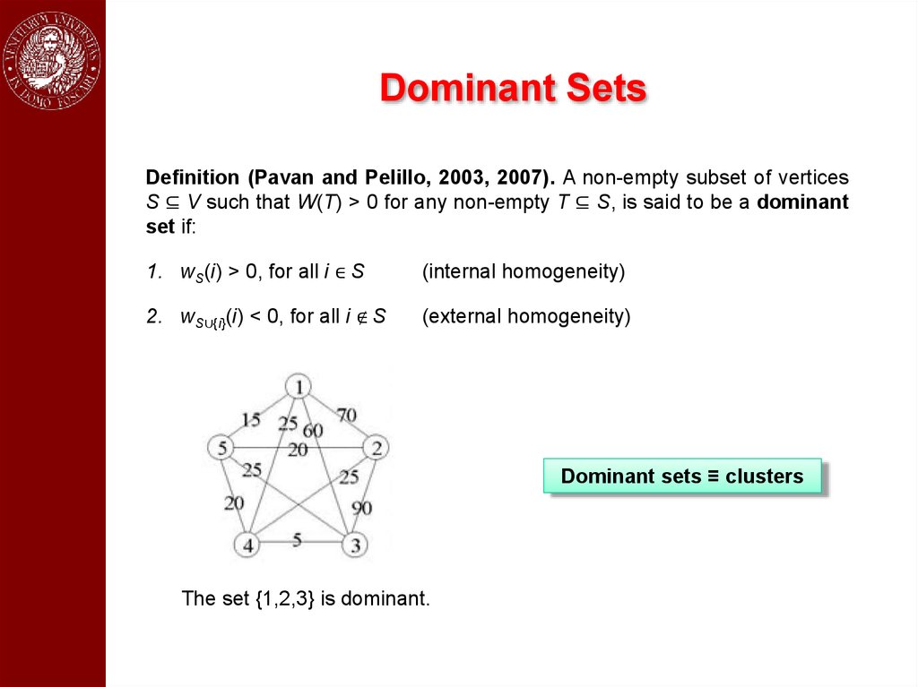
Dominant Sets
Definition (Pavan and Pelillo, 2003, 2007). A non-empty subset of vertices
S ⊆ V such that W(T) > 0 for any non-empty T ⊆ S, is said to be a dominant
set if:
1. wS(i) > 0, for all i ∈ S
(internal homogeneity)
2. wS∪{i}(i) < 0, for all i ∉ S
(external homogeneity)
Dominant sets ≡ clusters
The set {1,2,3} is dominant.

19.

The Clustering Game
Consider the following “clustering game.”
Assume a preexisting set of objects O and a (possibly asymmetric)
matrix of affinities A between the elements of O.
Two players play by simultaneously selecting an element of O.
After both have shown their choice, each player receives a payoff
proportional to the affinity that the chosen element has wrt the element
chosen by the opponent.
Clearly, it is in each player’s interest to pick an element that is strongly
supported by the elements that the adversary is likely to choose.
Hence, in the (pairwise) clustering game:
There are 2 players (because we have pairwise affinities)
The objects to be clustered are the pure strategies
The (null-diagonal) affinity matrix coincides with the similarity matrix

20.

Dominant Sets are ESS’s
Theorem (Torsello, Rota Bulò and Pelillo, 2006). Evolutionary stable
strategies of the clustering game with affinity matrix A are in a one-to-one
correspondence with dominant sets.
Note. Generalization of well-known Motzkin-Straus theorem from graph
theory (1965).
Dominant-set clustering
To get a single dominant-set cluster use, e.g., replicator dynamics (but
see Rota Bulò, Pelillo and Bomze, CVIU 2011, for faster dynamics)
To get a partition use a simple peel-off strategy: iteratively find a
dominant set and remove it from the graph, until all vertices have been
clustered
To get overlapping clusters, enumerate dominant sets (see Bomze, 1992;
Torsello, Rota Bulò and Pelillo, 2008)

21.

Special Case:
Symmetric Affinities
Given a symmetric real-valued matrix A (with null diagonal), consider the
following Standard Quadratic Programming problem (StQP):
maximize ƒ(x) = xTAx
subject to x∈∆
Note. The function ƒ(x) provides a measure of cohesiveness of a cluster
(see Pavan and Pelillo, 2003, 2007; Sarkar and Boyer, 1998; Perona and
Freeman, 1998).
ESS’s are in one-to-one correspondence
to (strict) local solutions of StQP
Note. In the 0/1 (symmetric) case, ESS’s are in one-to-one correspondence
to (strictly) maximal cliques (Motzkin-Straus theorem).

22.

Replicator Dynamics
Let xi(t) the population share playing pure strategy i at time t. The state of the
population at time t is: x(t)= (x1(t),…,xn(t))∈∆.
Replicator dynamics (Taylor and Jonker, 1978) are motivated by Darwin’s
principle of natural selection:
x˙ i
µ payoff of pure strategy i - average population payoff
xi
which yields:
x˙ i = xi [(Ax)i - xT Ax]
Theorem (Nachbar, 1990; Taylor and Jonker, 1978). A point x∈∆ is a
Nash equilibrium if and only if x is the limit point of a replicator dynamics
trajectory starting from the interior of ∆.
Furthermore, if x∈∆ is an ESS, then it is an asymptotically stable
equilibrium point for the replicator dynamics.

23.

Doubly Symmetric Games
In a doubly symmetric (or partnership) game, the payoff matrix A is
symmetric (A = AT).
Fundamental Theorem of Natural Selection (Losert and Akin,
1983).
For any doubly symmetric game, the average population payoff ƒ(x) =
xTAx is strictly increasing along any non-constant trajectory of
replicator dynamics, namely, d/dtƒ(x(t)) ≥ 0 for all t ≥ 0, with equality if
and only if x(t) is a stationary point.
Characterization of ESS’s (Hofbauer and Sigmund, 1988)
For any doubly simmetric game with payoff matrix A, the following
statements are equivalent:
a) x ∈ ∆ESS
b) x ∈ ∆ is a strict local maximizer of ƒ(x) = xTAx over the standard
simplex ∆
c) x ∈ ∆ is asymptotically stable in the replicator dynamics

24.

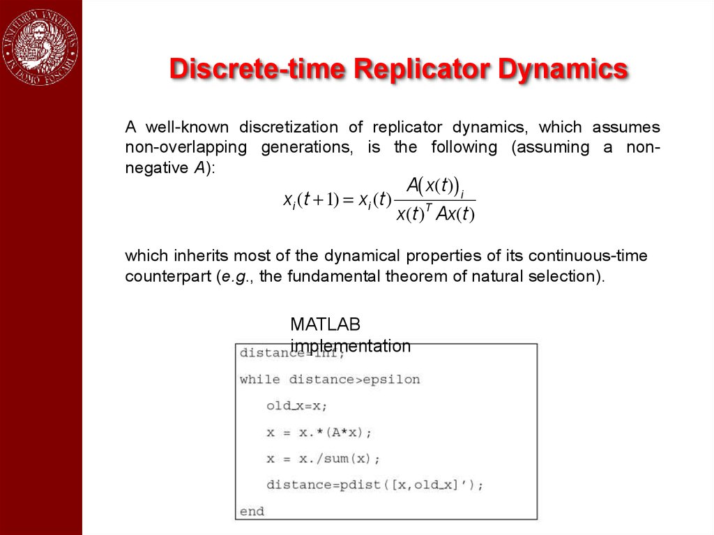
Discrete-time Replicator Dynamics
A well-known discretization of replicator dynamics, which assumes
non-overlapping generations, is the following (assuming a nonnegative A):
xi (t + 1) = xi (t)
A( x(t)) i
x(t)T Ax(t)
which inherits most of the dynamical properties of its continuous-time
counterpart (e.g., the fundamental theorem of natural selection).
MATLAB
implementation

25.

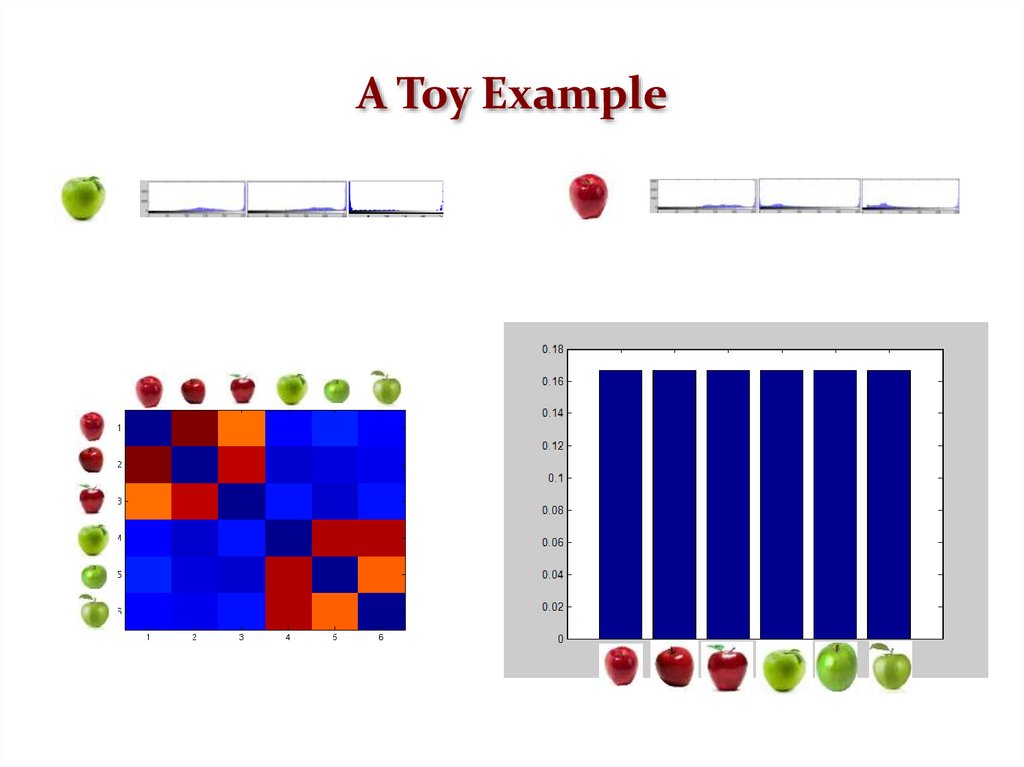
A Toy Example

26.

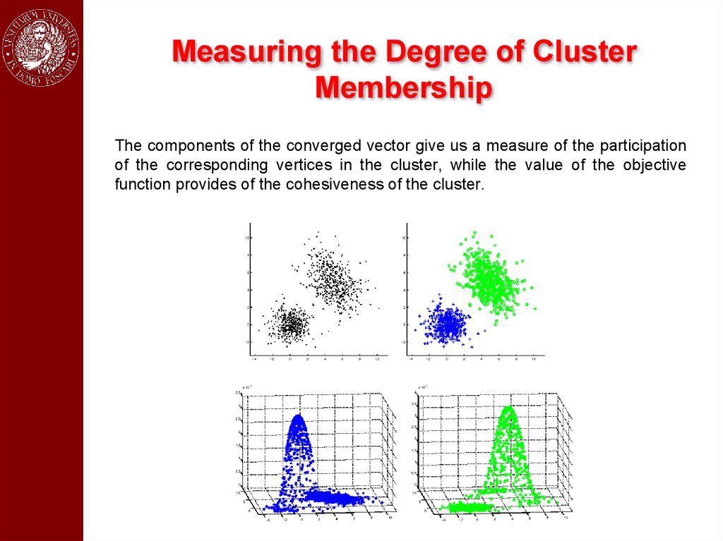
Measuring the Degree of Cluster
Membership
The components of the converged vector give us a measure of the participation
of the corresponding vertices in the cluster, while the value of the objective
function provides of the cohesiveness of the cluster.

27.

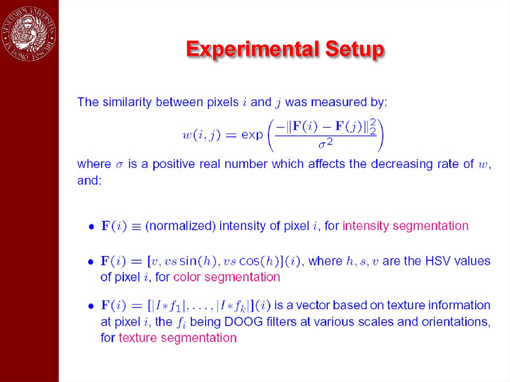
Application to Image Segmentation
An image is represented as an edge-weighted undirected graph, where
vertices correspond to individual pixels and edge-weights reflect the
“similarity” between pairs of vertices.
For the sake of comparison, in the experiments we used the same
similarities used in Shi and Malik’s normalized-cut paper (PAMI 2000).
To find a hard partition, the following peel-off strategy was used:
Partition_into_dominant_sets(G)
Repeat
find a dominant set
remove it from graph
until all vertices have been clustered
To find a single dominant set we used replicator dynamics (but see Rota
Bulò, Pelillo and Bomze, CVIU 2011, for faster game dynamics).

28.

Experimental Setup

29.

Intensity Segmentation Results
Dominant sets
Ncut

30.

Intensity Segmentation Results
Dominant sets
Ncut

31.

Results on the Berkeley Dataset
Dominant sets
Ncut

32.

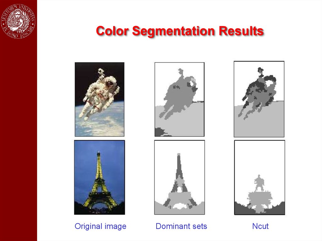
Color Segmentation Results
Original image
Dominant sets
Ncut

33.

Results on the Berkeley Dataset
Dominant sets
Ncut

34.

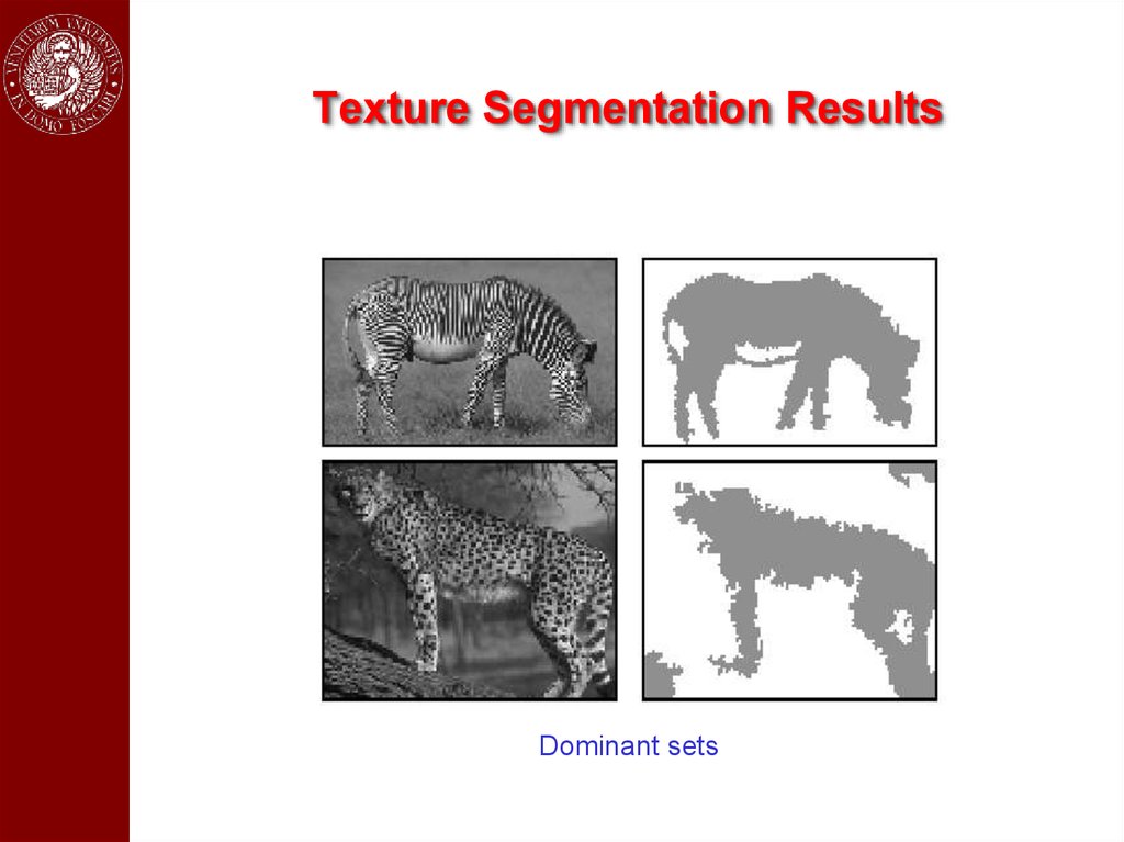
Texture Segmentation Results
Dominant sets

35.

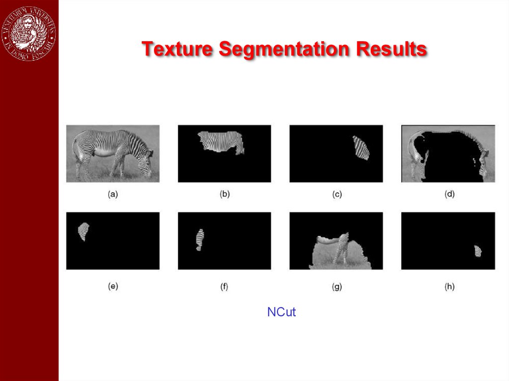
Texture Segmentation Results
NCut

36.

37.

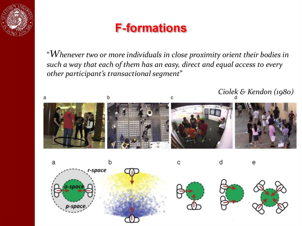
F-formations
“Whenever two or more individuals in close proximity orient their bodies in
such a way that each of them has an easy, direct and equal access to every
other participant’s transactional segment”
Ciolek & Kendon (1980)

38.

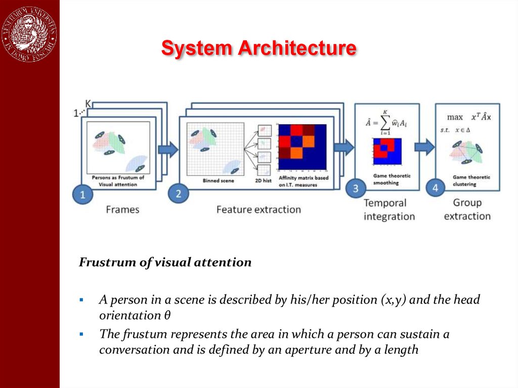
System Architecture
Frustrum of visual attention
A person in a scene is described by his/her position (x,y) and the head
orientation θ
The frustum represents the area in which a person can sustain a
conversation and is defined by an aperture and by a length

39.

Results
Spectral
Clustering

40.

Results
Qualitative results on the CoffeeBreak dataset compared with the state of the art
HFF.
Yellow = ground truth
Green = our method
Red = HFF.

41.

Other Applications of Dominant-Set
Clustering
Bioinformatics
Identification of protein binding sites (Zauhar and Bruist, 2005)
Clustering gene expression profiles (Li et al, 2005)
Tag Single Nucleotide Polymorphism (SNPs) selection (Frommlet, 2010)
Security and video surveillance
Detection of anomalous activities in video streams (Hamid et al., CVPR’05; AI’09)
Detection of malicious activities in the internet (Pouget et al., J. Inf. Ass. Sec. 2006)
Detection of F-formations (Hung and Kröse, 2011)
Content-based image retrieval
Wang et al. (Sig. Proc. 2008); Giacinto and Roli (2007)
Analysis of fMRI data
Neumann et al (NeuroImage 2006); Muller et al (J. Mag Res Imag. 2007)
Video analysis, object tracking, human action recognition
Torsello et al. (EMMCVPR’05); Gualdi et al. (IWVS’08); Wei et al. (ICIP’07)
Feature selection
Hancock et al. (GbR’11; ICIAP’11; SIMBAD’11)
Image matching and registration
Torsello et al. (IJCV 2011, ICCV’09, CVPR’10, ECCV’10)

42.

Extensions

43. Finding Overlapping Classes

First idea: run replicator dynamics from different starting points in the
simplex.
Problem: computationally expensive and no guarantee to find them
all.

44. Finding Overlapping Classes: Intuition

45. Building a Hierarchy: A Family of Quadratic Programs

46. The effects of α

47. The Landscape of fα

48. Sketch of the Hierarchical Clustering Algorithm

49.

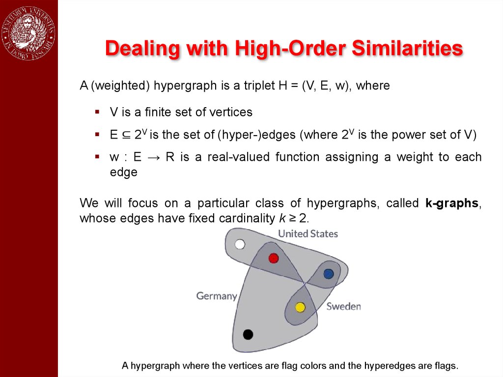
Dealing with High-Order Similarities
A (weighted) hypergraph is a triplet H = (V, E, w), where
V is a finite set of vertices
E ⊆ 2V is the set of (hyper-)edges (where 2V is the power set of V)
w : E → R is a real-valued function assigning a weight to each
edge
We will focus on a particular class of hypergraphs, called k-graphs,
whose edges have fixed cardinality k ≥ 2.
A hypergraph where the vertices are flag colors and the hyperedges are flags.

50.

The Hypergraph Clustering Game
Given a weighted k-graph representing an instance of a hypergraph
clustering problem, we cast it into a k-player (hypergraph) clustering
game where:
There are k players
The objects to be clustered are the pure strategies
The payoff function is proportional to the similarity of the
objects/strategies selected by the players
Definition (ESS-cluster). Given an instance of a hypergraph
clustering problem H = (V,E,w), an ESS-cluster of H is an ESS of
the corresponding hypergraph clustering game.
Like the k=2 case, ESS-clusters do incorporate both internal and
external cluster criteria (see PAMI 2013)

51.

ESS’s and Polynomial Optimization

52.

Baum-Eagon Inequality

53.

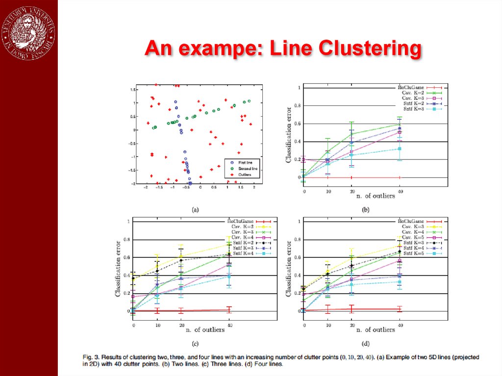
An exampe: Line Clustering

54.

In a nutshell…
The game-theoretic/dominant-set approach:
makes no assumption on the structure of the affinity matrix, being it able to
work with asymmetric and even negative similarity functions
does not require a priori knowledge on the number of clusters (since it
extracts them sequentially)
leaves clutter elements unassigned (useful, e.g., in figure/ground separation
or one-class clustering problems)
allows principled ways of assigning out-of-sample items (NIPS’04)
allows extracting overlapping clusters (ICPR’08)
generalizes naturally to hypergraph clustering problems, i.e., in the
presence of high-order affinities, in which case the clustering game is
played by more than two players (PAMI’13)
extends to hierarchical clustering (ICCV’03: EMMCVPR’09)
allows using multiple affinity matrices using Pareto-Nash notion
(SIMBAD’15)

55.

References
S. Rota Bulò and M. Pelillo. Dominant-set clustering: A review.
Europ. J. Oper. Res. (2017)
M. Pavan and M. Pelillo. Dominant sets and pairwise clustering. PAMI
2007.
M. Pavan and M. Pelillo. Dominant sets and hierarchical clustering.
ICCV 2003.
M. Pavan and M. Pelillo. Efficient out-of-sample extension of dominantset clusters. NIPS 2004.
A. Torsello, S. Rota Bulò and M. Pelillo. Grouping with asymmetric
affinities: A game-theoretic perspective. CVPR 2006.
A. Torsello, S. Rota Bulò and M. Pelillo. Beyond partitions: Allowing
overlapping groups in pairwise clustering. ICPR 2008.
S. Rota Bulò and M. Pelillo. A game-theoretic approach to hypergraph
clustering. PAMI’13.
S. Rota Bulò, M. Pelillo and I. M. Bomze. Graph-based quadratic
optimization: A fast evolutionary approach. CVIU 2011.

56. Hume-Nash Machines Context-Aware Models of Learning and Recognition

57.

Machine learning:
The standard paradigm
From: Duda, Hart and Stork, Pattern Classification (2000)

58.

Limitations
There are cases where it’s not easy to find satisfactory feature-vector
representations.
Some examples
when experts cannot define features in a straightforward way
when data are high dimensional
when features consist of both numerical and categorical
variables,
in the presence of missing or inhomogeneous data
when objects are described in terms of structural properties
…

59.

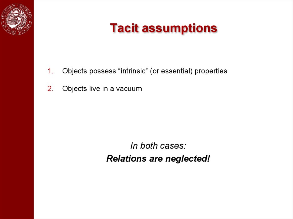
Tacit assumptions
1.
Objects possess “intrinsic” (or essential) properties
2.
Objects live in a vacuum
In both cases:
Relations are neglected!

60.

The many types of relations
Similarity relations between objects
Similarity relations between categories
Contextual relations
…
Application domains: Natural language processing, computer
vision, computational biology, adversarial contexts, social signal
processing, medical image analysis, social network analysis,
network medicine, …

61.

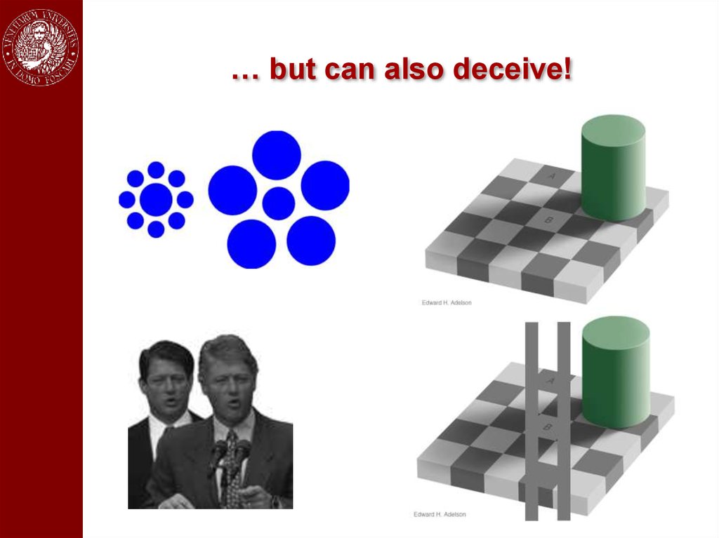
Context helps …

62.

… but can also deceive!

63.

Context and the brain
From: M. Bar, “Visual objects in context”, Nature Reviews Neuroscience, August 2004.

64.

Beyond features?
The field is showing an increasing propensity towards relational
approaches, e.g.,
Kernel methods
Pairwise clustering (e.g., spectral methods, game-theoretic
methods)
Graph transduction
Dissimilarity representations (Duin et al.)
Theory of similarity functions (Blum, Balcan, …)
Relational / collective classification
Graph mining
Contextual object recognition
…
See also “link analysis” and the parallel development of “network
science” …

65.

The SIMBAD project
1.
University of Venice (IT), coordinator
2.
University of York (UK)
3.
Technische Universität Delft (NL)
4.
Insituto Superior Técnico, Lisbon (PL)
5.
University of Verona (IT)
6.
ETH Zürich (CH)
http://simbad-fp7.eu

66.

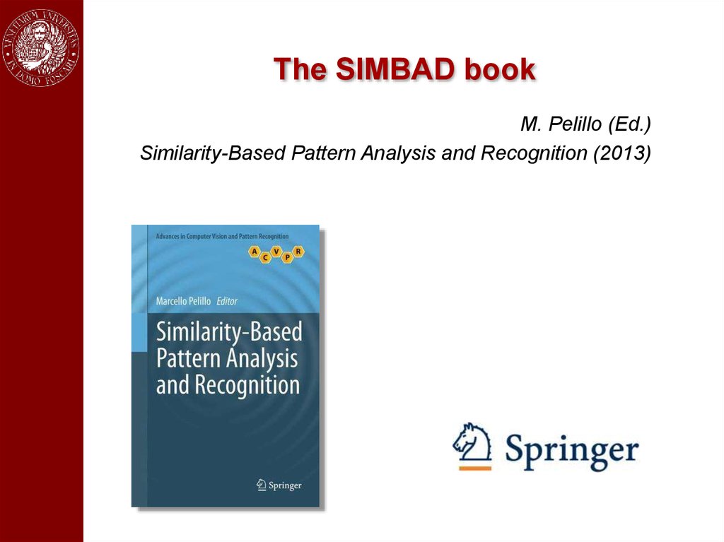
The SIMBAD book
M. Pelillo (Ed.)
Similarity-Based Pattern Analysis and Recognition (2013)

67.

Challenges to similarity-based
approaches
Departing from vector-space representations:
• dealing with (dis)similarities that might not possess the
Euclidean behavior or not even obey the requirements of a
metric
• lack of Euclidean and/or metric properties undermines the
foundations of traditional pattern recognition algorithms
The customary approach to
(dis)similarities is embedding.
deal
with
non-(geo)metric
• based on the assumption that the non-geometricity of similarity
information can be eliminated or somehow approximated away
• when there is significant information content in the nongeometricity of the data, alternative approaches are needed

68.

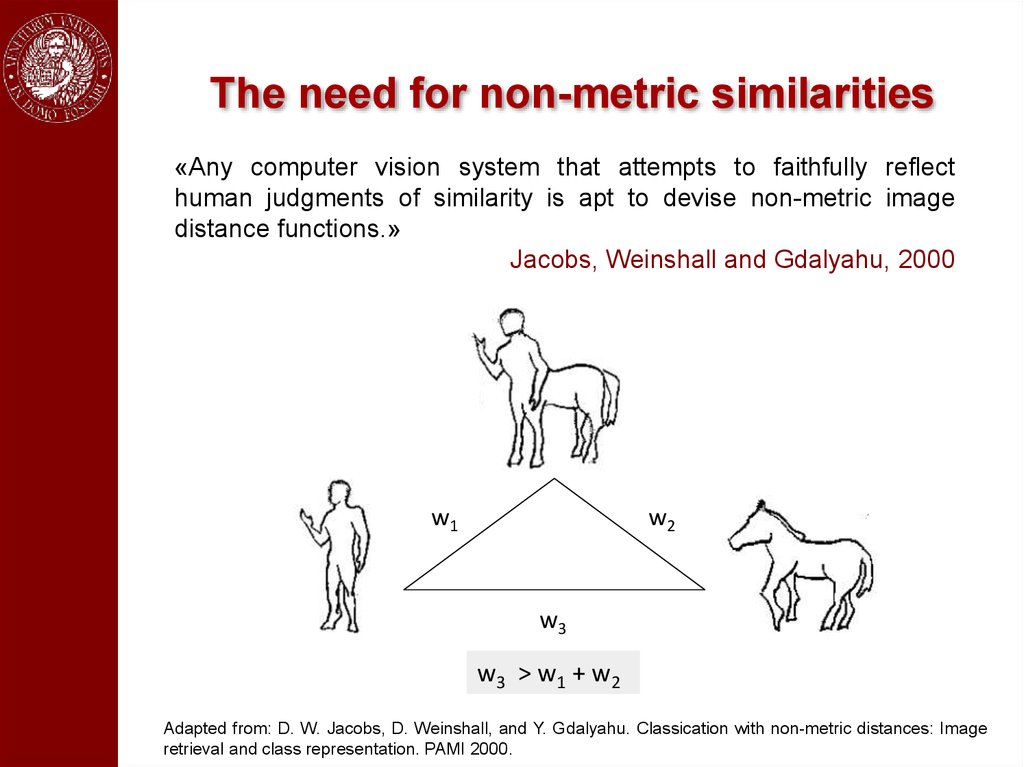
The need for non-metric similarities
«Any computer vision system that attempts to faithfully reflect
human judgments of similarity is apt to devise non-metric image
distance functions.»
Jacobs, Weinshall and Gdalyahu, 2000
w1
w2
w3
w3 > w1 + w2
Adapted from: D. W. Jacobs, D. Weinshall, and Y. Gdalyahu. Classication with non-metric distances: Image
retrieval and class representation. PAMI 2000.

69.

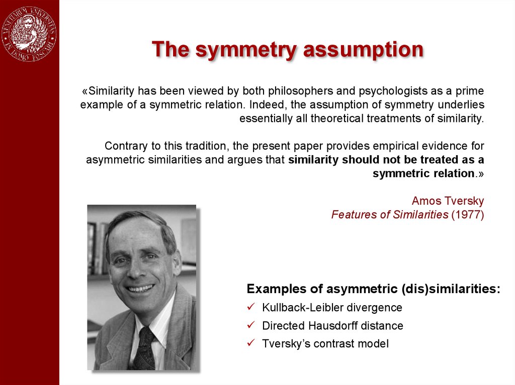
The symmetry assumption
«Similarity has been viewed by both philosophers and psychologists as a prime
example of a symmetric relation. Indeed, the assumption of symmetry underlies
essentially all theoretical treatments of similarity.
Contrary to this tradition, the present paper provides empirical evidence for
asymmetric similarities and argues that similarity should not be treated as a
symmetric relation.»
Amos Tversky
Features of Similarities (1977)
Examples of asymmetric (dis)similarities:
Kullback-Leibler divergence
Directed Hausdorff distance
Tversky’s contrast model

70.

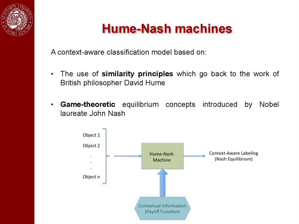
Hume-Nash machines
A context-aware classification model based on:
• The use of similarity principles which go back to the work of
British philosopher David Hume
• Game-theoretic equilibrium concepts introduced by Nobel
laureate John Nash

71.

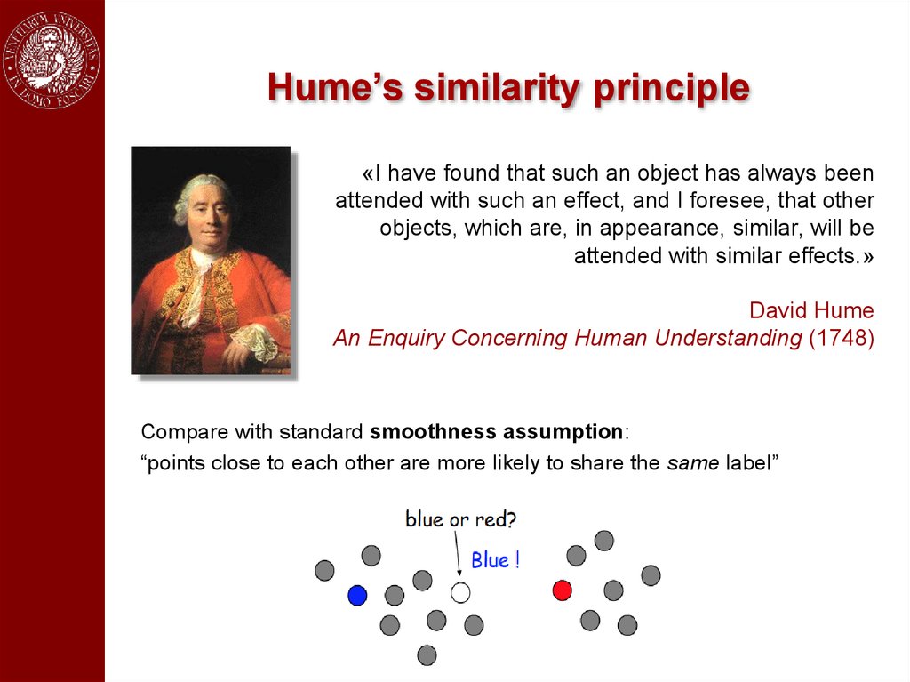
Hume’s similarity principle
«I have found that such an object has always been
attended with such an effect, and I foresee, that other
objects, which are, in appearance, similar, will be
attended with similar effects.»
David Hume
An Enquiry Concerning Human Understanding (1748)
Compare with standard smoothness assumption:
“points close to each other are more likely to share the same label”

72.

Why game theory?
Answer #1:
Because it works! (well, great…)
Answer #2:
Because it allows us to naturally deal with context-aware problems,
non-Euclidean, non-metric, high-order, and whatever-you-like
(dis)similarities
Answer #3:
Because it allows us to model in a principled way problems not
formulable in terms of simgle-objective optimization principles

73.

The (Consistent) labeling problem
A labeling problem involves:
A set of n objects B = {b1,…,bn}
A set of m labels Λ = {1,…,m}
The goal is to label each object of B with a label of Λ.
To this end, two sources of information are exploited:
Local measurements which capture the salient features of each
object viewed in isolation
Contextual information, expressed in terms of a real-valued n2 x
m2 matrix of compatibility coefficients R = {rij(λ,μ)}.
The coefficient rij(λ,μ) measures the strenght of compatibility between
the two hypotheses: “bi is labeled λ” and “bj is labeled μ“.

74.

Relaxation labeling processes
In a now classic 1976 paper, Rosenfeld, Hummel, and Zucker
introduced the following update rule (assuming a non-negative
compatibility matrix):
(t +1)
i
p
p(ti ) ( l)q(ti ) (l )
( l) =
å p(ti ) (m)q(ti ) (m)
m
where
q(ti ) ( l) = å å rij (l, m) p(ti ) (m)
j
m
quantifies the support that context gives at time t to the
hypothesis “bi is labeled with label λ”.
See (Pelillo, 1997) for a rigorous derivation of this rule in the
context of a formal theory of consistency.

75.

Applications
Since their introduction in the mid-1970’s relaxation labeling
algorithms have found applications in virtually all problems in
computer vision and pattern recognition:
Edge and curve detection and enhancement
Region-based segmentation
Stereo matching
Shape and object recognition
Grouping and perceptual organization
Graph matching
Handwriting interpretation
…
Further, intriguing similarities exist between relaxation labeling
processes and certain mechanisms in the early stages of biological
visual systems (see Zucker, Dobbins and Iverson, 1989)

76.

Hummel and Zucker’s consistency
In 1983, Hummel and Zucker developed an elegant theory of
consistency in labeling problem.
By analogy with the unambiguous case, which is easily
understood, they define a weighted labeling assignment p
consistent if:
å p (l)q (l) ³ åv (l)q (l)
i
l
i
i
i
i =1… n
l
for all labeling assignments v.
If strict inequalities hold for all v ≠ p, then p is said to be strictly
consistent.
Geometrical interpretation.
The support vector q points
away from all tangent vectors at
p (it has null projection in IK).

77.

Relaxation labeling as
non-cooperative Games
As observed by Miller and Zucker (1991) the consistent labeling
problem is equivalent to a non-cooperative game.
Indeed, in such formulation we have:
Objects = players
Labels = pure strategies
Weighted labeling assignments = mixed strategies
Compatibility coefficients = payoffs
and:
Consistent labeling = Nash equilibrium
Further, the Rosenfeld-Hummel-Zucker update rule corresponds to
discrete-time multi-population replicator dynamics.

78.

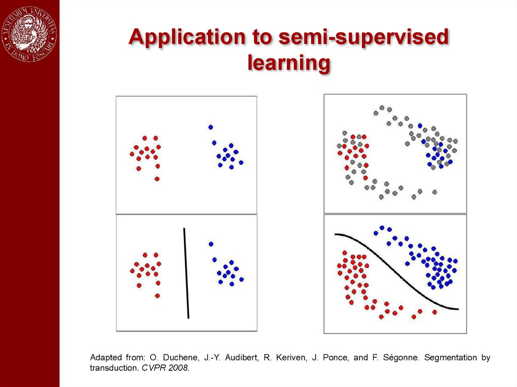
Application to semi-supervised
learning
Adapted from: O. Duchene, J.-Y. Audibert, R. Keriven, J. Ponce, and F. Ségonne. Segmentation by
transduction. CVPR 2008.

79.

Graph transduction
Given a set of data points grouped into:
labeled data:
unlabeled
data:
Express data as a graph G=(V,E)
V : nodes representing labeled and unlabeled points
E : pairwise edges between nodes weighted by the similarity
between the corresponding pairs of points
Goal: Propagate the information available at the labeled nodes to
unlabeled ones in a “consistent” way.
Cluster assumption:
The data form distinct clusters
Two points in the same cluster are expected to be in the same
class

80.

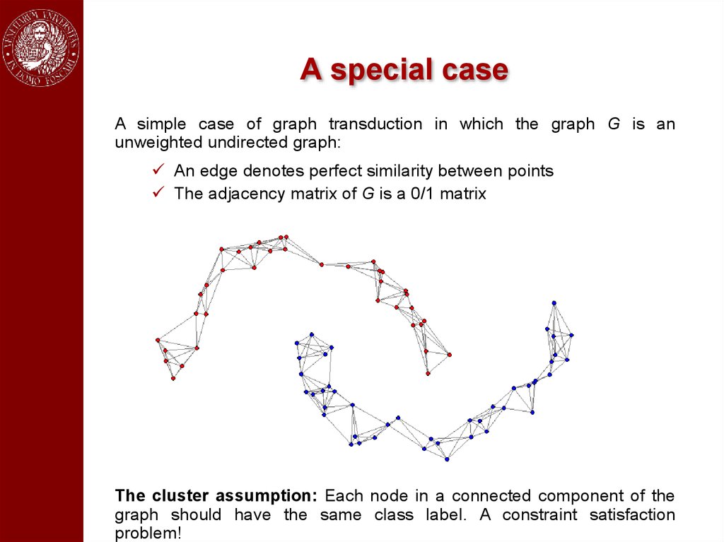
A special case
A simple case of graph transduction in which the graph G is an
unweighted undirected graph:
An edge denotes perfect similarity between points
The adjacency matrix of G is a 0/1 matrix
The cluster assumption: Each node in a connected component of the
graph should have the same class label. A constraint satisfaction
problem!

81.

The graph transduction game
Given a weighted graph G = (V, E, w), the graph trasduction game is as
follow:
Nodes = players
Labels = pure strategies
Weighted labeling assignments = mixed strategies
Compatibility coefficients = payoffs
The transduction game is in fact played among the unlabeled players to
choose their memberships.
Consistent labeling = Nash equilibrium
Can be solved used standard relaxation labeling / replicator dynamics.
Applications: NLP (see next part), interactive image segmentation,
content-based image retrieval, people tracking and re-identification, etc.

82.

In short…
Graph transduction can be formulated as a non-cooperative game
(i.e., a consistent labeling problem).
The proposed game-theoretic framework can cope with symmetric,
negative and asymmetric similarities (none of the existing
techniques is able to deal with all three types of similarities).
Experimental results on standard datasets show that our approach is
not only more general but also competitive with standard
approaches.
A. Erdem and M. Pelillo. Graph transduction as a noncooperative
game. Neural Computation 24(3) (March 2012).

83.

Extensions
The approach described here is being naturally extended along
several directions:
Using more powerful algorithms than “plain” replicator dynamics
(e.g., Porter et al., 2008; Rota Bulò and Bomze, 2010)
Dealing with high-order interactions (i.e., hypergraphs) (e.g.,
Agarwal et al., 2006; Rota Bulò and Pelillo, 2013)
From the “homophily” to the “Hume” similarity principle
-> “similar objects should be assigned similar labels”
Introducing uncertainty in “labeled” players

84.

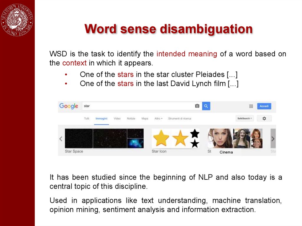
Word sense disambiguation
WSD is the task to identify the intended meaning of a word based on
the context in which it appears.
One of the stars in the star cluster Pleiades [...]
One of the stars in the last David Lynch film [...]
Cinema
It has been studied since the beginning of NLP and also today is a
central topic of this discipline.
Used in applications like text understanding, machine translation,
opinion mining, sentiment analysis and information extraction.

85.

Approaches
Supervised approaches
Use sense labeled corpora to build
classifiers.
Semi-supervised approaches
Use transductive methods to transfer the
information from few labeled words to
unlabeled.
Unsupervised approaches
Use a knowledge base to collect all the
senses of a given word.
Exploit contextual information to choose
the best sense for each word.

86.

WSD games
The WSD problem can be formulated in game-theoretic terms modeling:
the players of the games as the words to be disambiguated.
the strategies of the games as the senses of each word.
the payoff matrices of each game as a sense similarity function.
the interactions among the players as a weighted graph.
Nash equilibria correspond to consistent word-sense assignments!
Word-level similarities: proportional to strength of co-occurrence
between words
Sense-level similarities: computed using WordNet / BabelNet
ontologies
R. Tripodi and M. Pelillo. A game-theoretic approach to word sense
disambiguation. Computational Linguistics 43(1) (January 2017).

87.

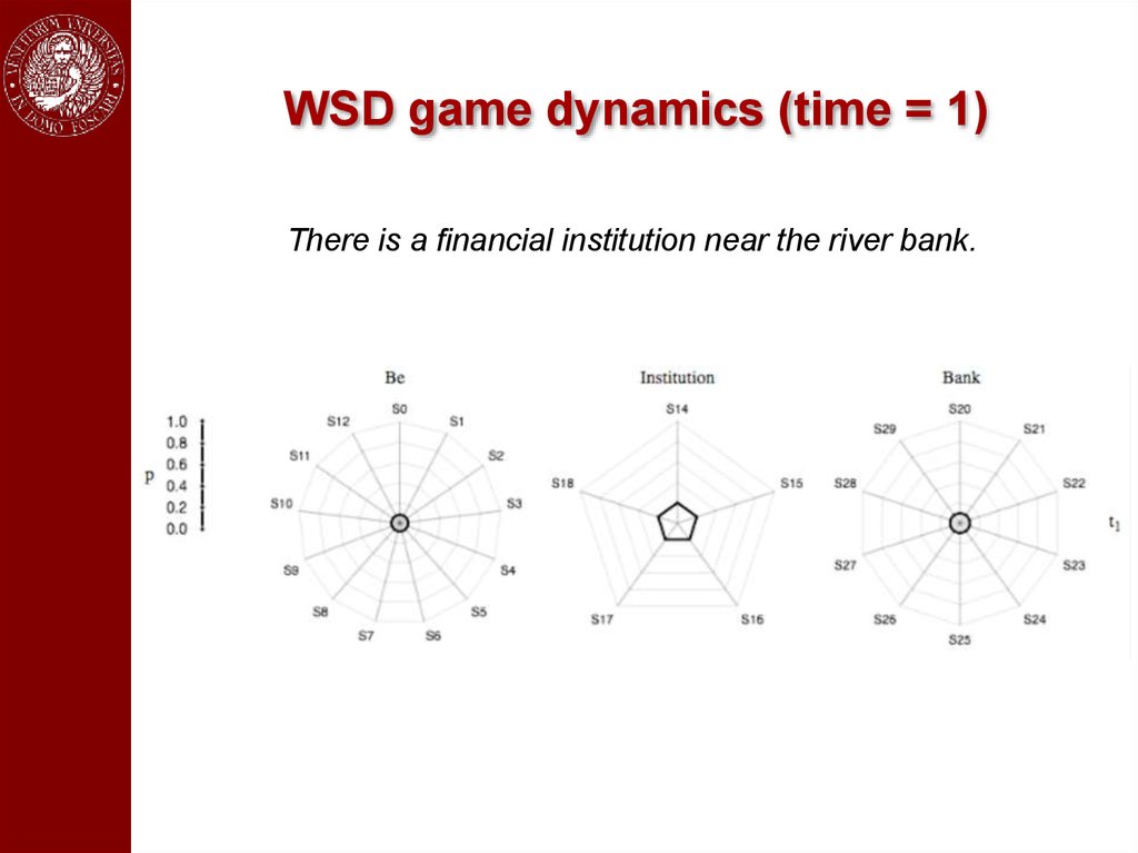
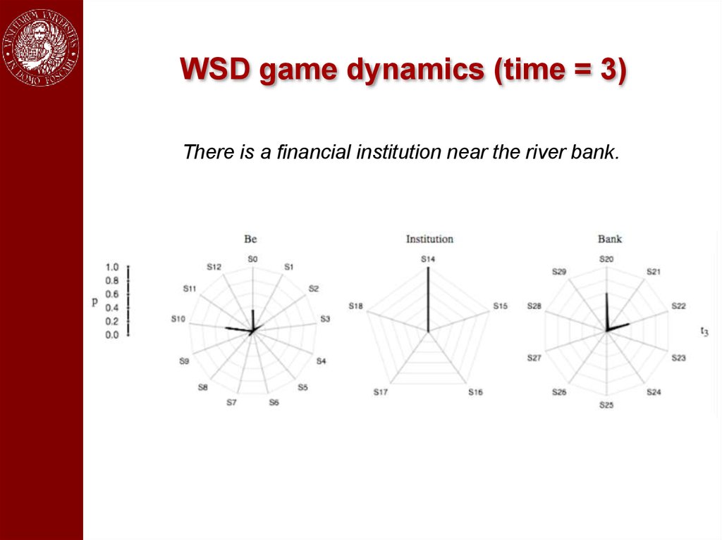
An example
There is a financial institution near the river bank.

88.

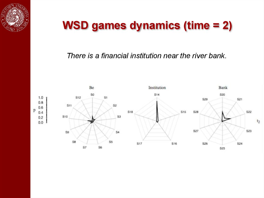
WSD game dynamics (time = 1)
There is a financial institution near the river bank.

89.

WSD games dynamics (time = 2)
There is a financial institution near the river bank.

90.

WSD game dynamics (time = 3)
There is a financial institution near the river bank.

91.

WSD games dynamics (time = 12)
There is a financial institution near the river bank.

92.

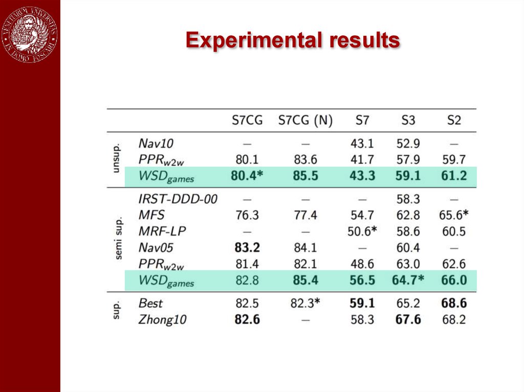
Experimental setup

93.

Experimental results

94.

Experimental results (entity linking)

95.

To sum up
Game theory offers a principled and viable solution to context-aware
pattern recognition problems, based on the idea of dynamical
competition among hypotheses driven by payoff functions.
Distiguishing features:
• No restriction imposed on similarity/payoff function (unlike, e.g.,
spectral methods)
• Shifts the emphasis from optima of objective functions to equilibria
of dynamical systems.
On-going work:
• Learning payoff functions from data (Pelillo and Refice, 1994)
• Combining Hume-Nash machines with deep neural networks
• Applying them to computer vision problems such as scene parsing,
object recognition, video analysis

96.

References
A. Rosenfeld, R. A. Hummel, and S. W. Zucker. Scene labeling by relaxation
operations. IEEE Trans. Syst. Man. Cybern (1976)
R. A. Hummel and S. W. Zucker. On the foundations of relaxation labeling
processes. IEEE Trans. Pattern Anal. Machine Intell. (1983)
M. Pelillo. The dynamics of nonlinear relaxation labeling processes. J. Math.
Imaging and Vision (1997)
D. A. Miller and S. W. Zucker. Copositive-plus Lemke algorithm solves
polymatrix games. Operation Research Letters (1991)
A. Erdem and M. Pelillo. Graph transduction as a non-cooperative game.
Neural Computation (2012)
R. Tripodi and M. Pelillo. A game-theoretic approach to word-sense
disambiguation. Computational Linguistics (2017)
M. Pelillo and M. Refice. Learning compatibility coefficients for relaxation
labeling processes. IEEE Trans. Pattern Anal. Machine Intell. (1994)
S. Rota Bulò and M. Pelillo. Dominant-set clustering: A review. Europ. J. Oper.
Res. (2017)

97. Capturing Elongated Structures / 1

98. Capturing Elongated Structures / 2

99.

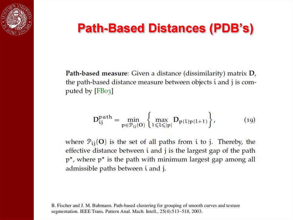
Path-Based Distances (PDB’s)
B. Fischer and J. M. Buhmann. Path-based clustering for grouping of smooth curves and texture
segmentation. IEEE Trans. Pattern Anal. Mach. Intell., 25(4):513–518, 2003.

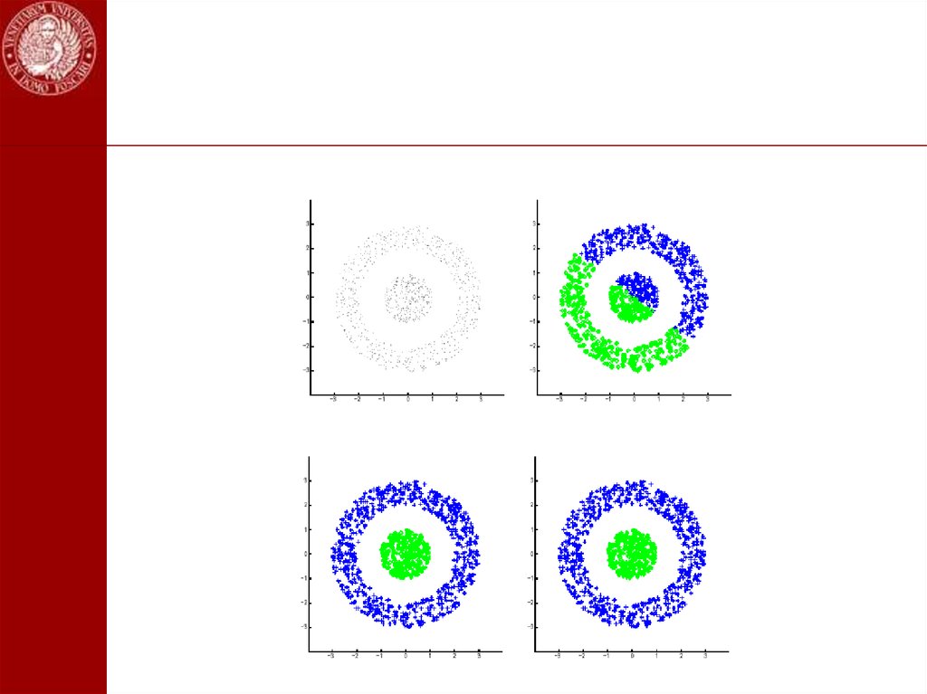
100. Example: Without PBD (σ = 2)

101. Example: Without PDB (σ = 4)

102. Example: Without PDB (σ = 8)

103. Example: With PDB (σ = 0.5)

104.

105.

106.

Constrained Dominant Sets
Let A denote the (weighted) adjacency matrix of a graph G=(V,E). Given a subset
of vertices S V and a parameter > 0, define the following parameterized
family of quadratic programs:
where IS is the diagonal matrix whose diagonal elements are set to 1 in
correspondence to the vertices contained in V \ S, and to zero otherwise:
Property. By setting:
all local solutions will have a support containing elements of S.

107.

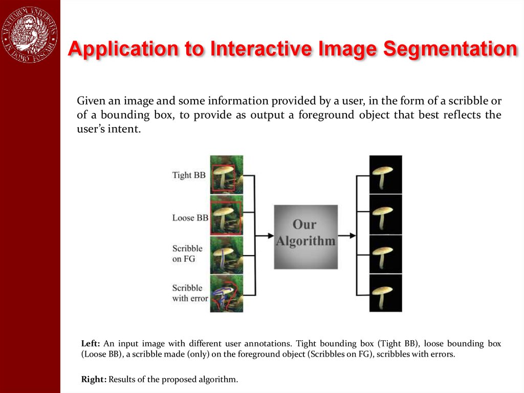
Application to Interactive Image Segmentation
Given an image and some information provided by a user, in the form of a scribble or
of a bounding box, to provide as output a foreground object that best reflects the
user’s intent.
Left: An input image with different user annotations. Tight bounding box (Tight BB), loose bounding box
(Loose BB), a scribble made (only) on the foreground object (Scribbles on FG), scribbles with errors.
Right: Results of the proposed algorithm.

108.

System Overview
Left: Over-segmented image with a user scribble (blue label).
Middle: The corresponding affinity matrix, using each over-segments as a node, showing its two
parts: S, the constraint set which contains the user labels, and V n S, the part of the graph which
takes the regularization parameter .
Right: RRp, starts from the barycenter and extracts the first dominant set and update x and M, for
the next extraction till all the dominant sets which contain the user labeled regions are extracted.

109.

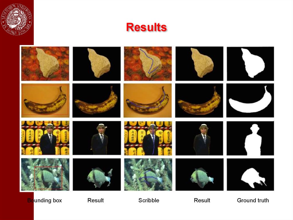
Results

110.

Results
Bounding box
Result
Scribble
Result
Ground truth

111.

Results
Bounding box
Result
Scribble
Result
Ground truth

112.

The “protein function predition”
game
Motivation: network-based methods for the automatic prediction of
protein functions can greatly benefit from exploiting both the
similarity between proteins and the similarity between functional
classes.
Hume’s principle:
functionalities
similar
proteins
should
have
similar
We envisage a (non-cooperative) game where
• Players = proteins,
• Strategies = functional classes
• Payoff function = combination of protein- and function-level
similarities
Nash equilibria turn out to provide consistent functional labelings of
proteins.

113.

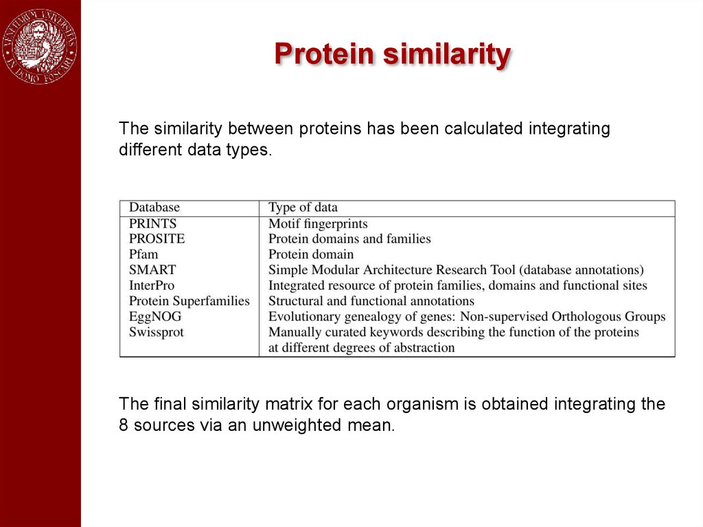
Protein similarity
The similarity between proteins has been calculated integrating
different data types.
The final similarity matrix for each organism is obtained integrating the
8 sources via an unweighted mean.

114.

Funtion similarity
The similarities between the classes
functionalities have been computed using
the Gene Ontology (GO)
The similarity between the GO terms for
each integrated network and each ontology
are computed using:
• semantic similarities measures (Resnick
or Lin)
• a Jaccard similarity measure between the
annotations of each GO term.

115.

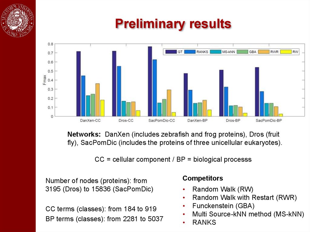
Preliminary results
Networks: DanXen (includes zebrafish and frog proteins), Dros (fruit
fly), SacPomDic (includes the proteins of three unicellular eukaryotes).
CC = cellular component / BP = biological processs
Number of nodes (proteins): from
3195 (Dros) to 15836 (SacPomDic)
CC terms (classes): from 184 to 919
BP terms (classes): from 2281 to 5037
Competitors
Random Walk (RW)
Random Walk with Restart (RWR)
Funckenstein (GBA)
Multi Source-kNN method (MS-kNN)
RANKS