Binary Search Trees

1. Binary Search Trees

SDP4

2. Binary Trees

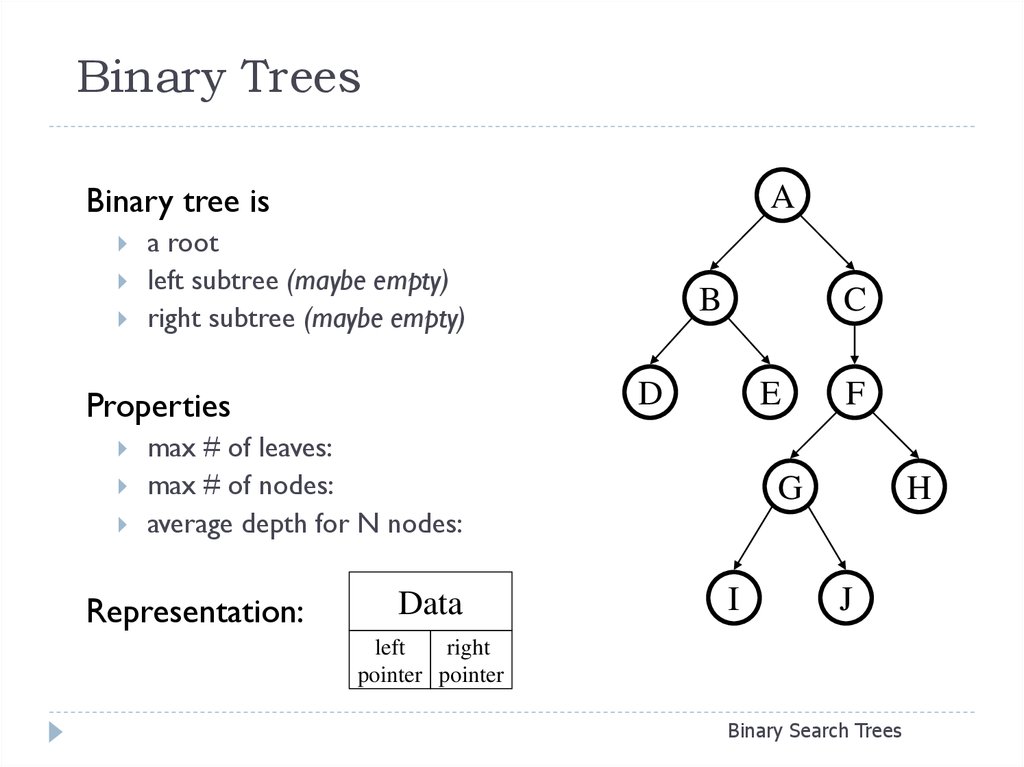
Binary tree is
A
a root
left subtree (maybe empty)
right subtree (maybe empty)
C
D
Properties
B
E
max # of leaves:
max # of nodes:
average depth for N nodes:
Representation:
Data
F
G
I
H
J
left
right
pointer pointer
Binary Search Trees

3.

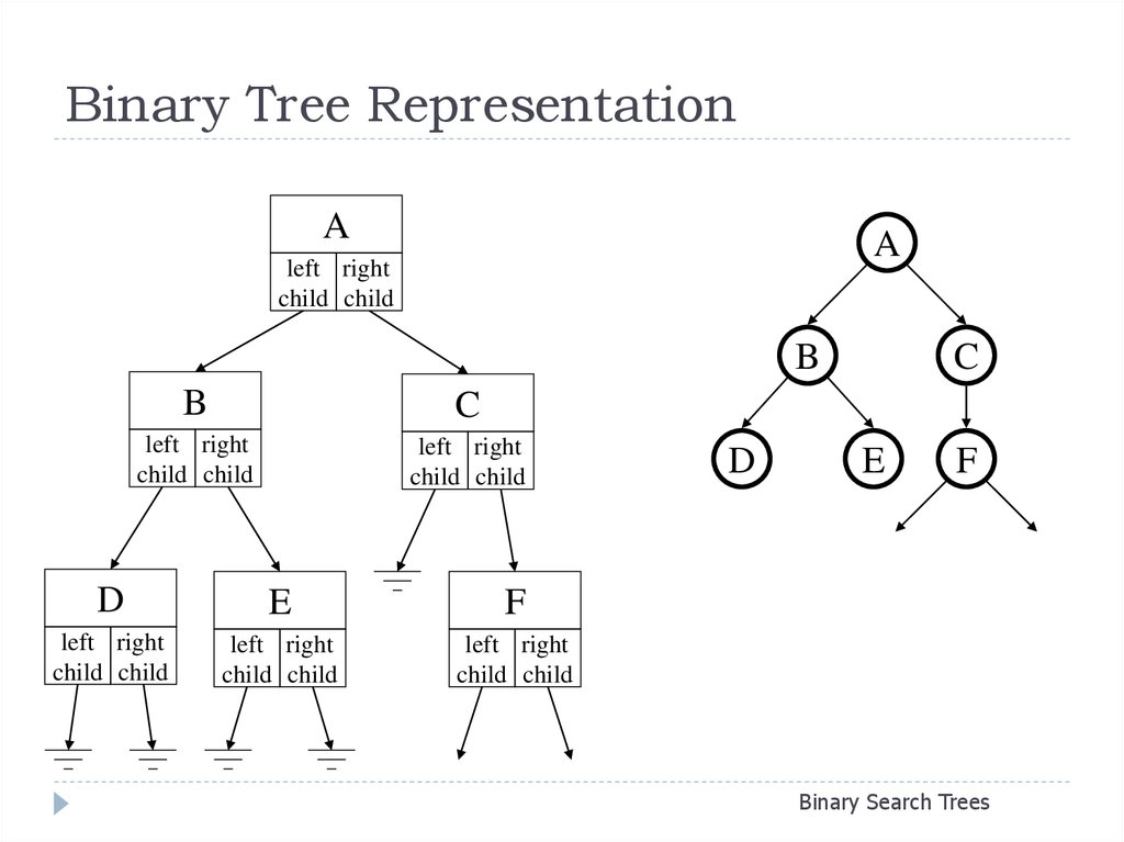
Binary Tree Representation
A
A
left right
child child
B
B
C
left right
child child
left right
child child
D
E
F
left right
child child
left right
child child
left right
child child
D
C
E
F
Binary Search Trees

4. Dictionary ADT

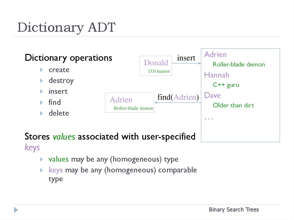
Dictionary operations
create
destroy
insert
find
delete
Donald
insert
l33t haxtor
Adrien
Roller-blade demon
Hannah
C++ guru
Adrien
find(Adrien) Dave
Roller-blade demon
Older than dirt
…
Stores values associated with user-specified
keys
values may be any (homogeneous) type
keys may be any (homogeneous) comparable
type
Binary Search Trees

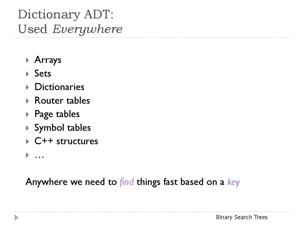
5. Dictionary ADT: Used Everywhere

Arrays
Sets
Dictionaries
Router tables
Page tables
Symbol tables
C++ structures
…
Anywhere we need to find things fast based on a key
Binary Search Trees

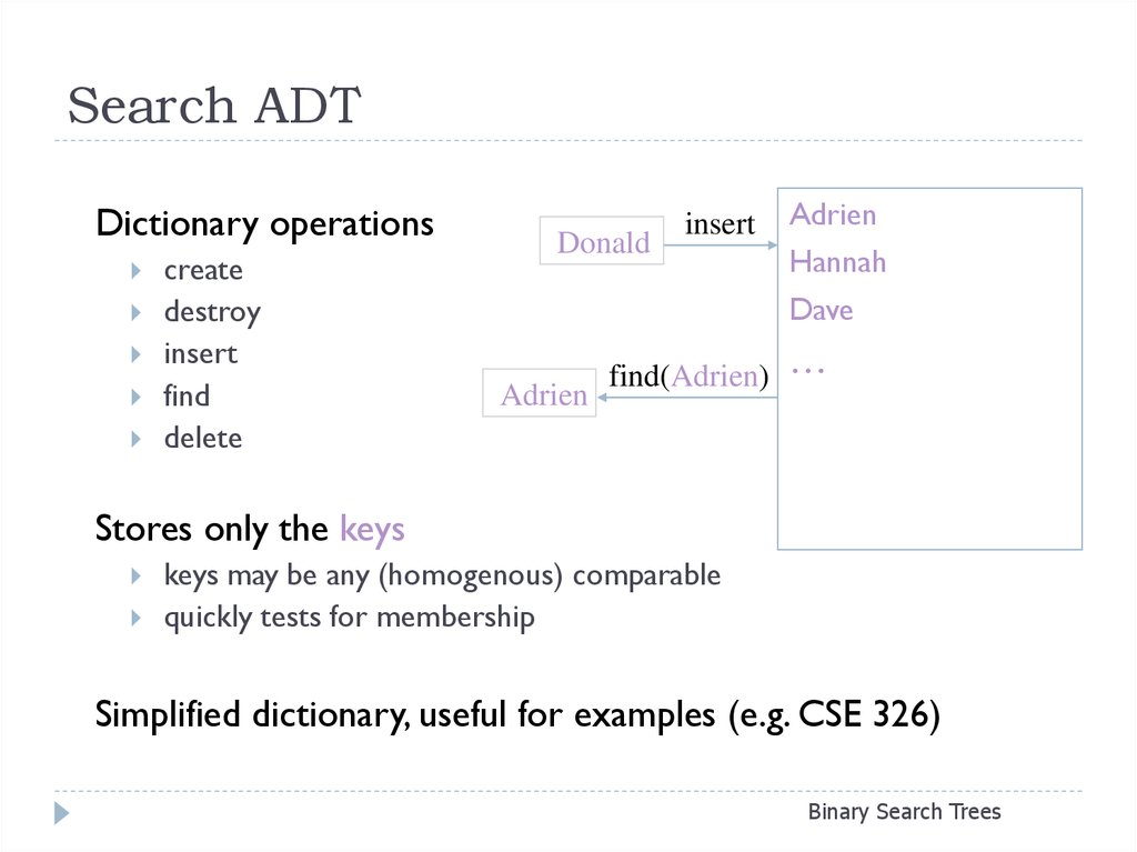
6. Search ADT

Dictionary operations
create
destroy
insert
find
delete
Donald
Adrien
insert
Adrien
Hannah
Dave
find(Adrien) …
Stores only the keys
keys may be any (homogenous) comparable
quickly tests for membership
Simplified dictionary, useful for examples (e.g. CSE 326)
Binary Search Trees

7. Dictionary Data Structure: Requirements

Fast insertion
Fast searching
runtime:
runtime:
Fast deletion
runtime:
Binary Search Trees

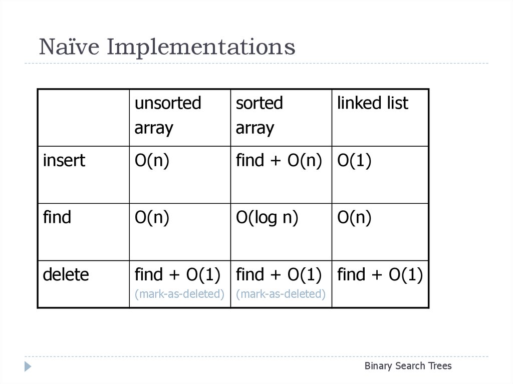
8. Naïve Implementations

unsorted
array
sorted
array
linked list
insert
O(n)
find + O(n) O(1)
find
O(n)
O(log n)
delete
find + O(1) find + O(1) find + O(1)
O(n)
(mark-as-deleted) (mark-as-deleted)
Binary Search Trees

9. Binary Search Tree Dictionary Data Structure

Binary tree property
Search tree property
8
each node has 2 children
result:
storage is small
operations are simple
average depth is small
all keys in left subtree smaller than
root’s key
all keys in right subtree larger than
root’s key
result:
easy to find any given key
Insert/delete by changing links
5
2
11
6
4
10
7
9
12
14
13
Binary Search Trees

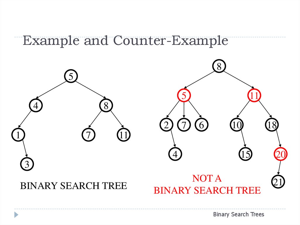
10. Example and Counter-Example

8
5
5
4
8
2
1
11
7
7
6
10
18
11
4
15
20
3
BINARY SEARCH TREE
NOT A
BINARY SEARCH TREE
Binary Search Trees
21

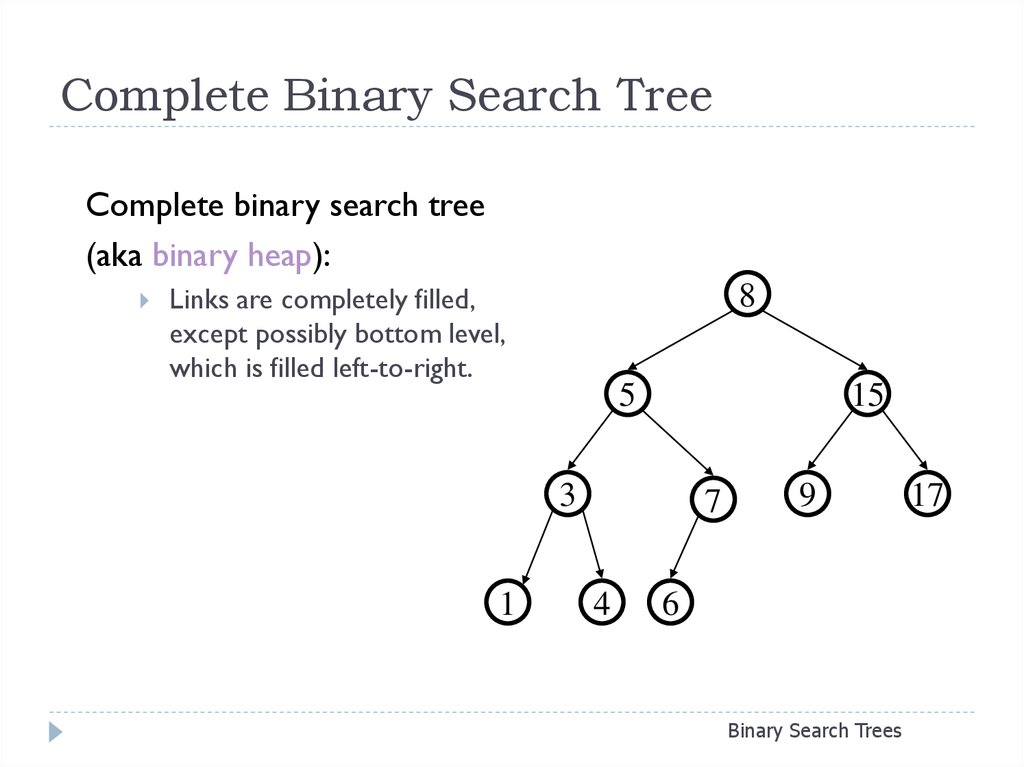
11. Complete Binary Search Tree

Complete binary search tree
(aka binary heap):
Links are completely filled,
except possibly bottom level,
which is filled left-to-right.
8
5
15
3
1
7
4
9
6
Binary Search Trees
17

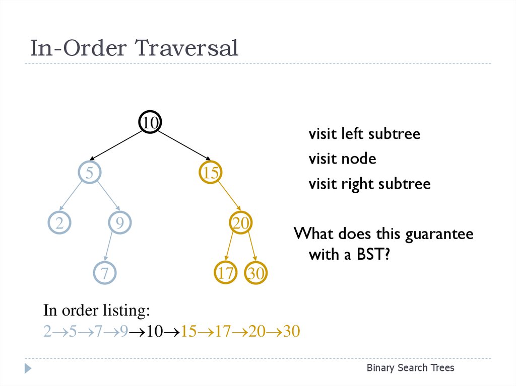
12. In-Order Traversal

10
5
visit left subtree
visit node
visit right subtree
15
2
9
7
20
What does this guarantee
with a BST?
17 30
In order listing:
2 5 7 9 10 15 17 20 30
Binary Search Trees

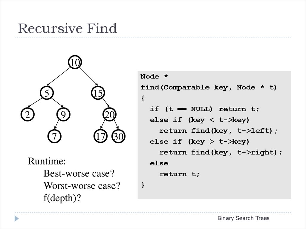
13. Recursive Find

10
5
15
2
9
7
20
17 30
Runtime:
Best-worse case?
Worst-worse case?
f(depth)?
Node *
find(Comparable key, Node * t)
{
if (t == NULL) return t;
else if (key < t->key)
return find(key, t->left);
else if (key > t->key)
return find(key, t->right);
else
return t;
}
Binary Search Trees

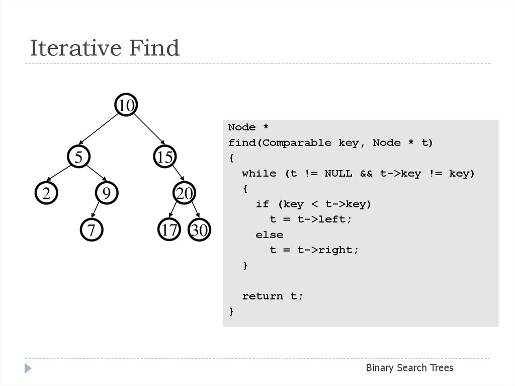
14. Iterative Find

10
5
15
2
9
7
20
17 30
Node *
find(Comparable key, Node * t)
{
while (t != NULL && t->key != key)
{
if (key < t->key)
t = t->left;
else
t = t->right;
}
return t;
}
Binary Search Trees

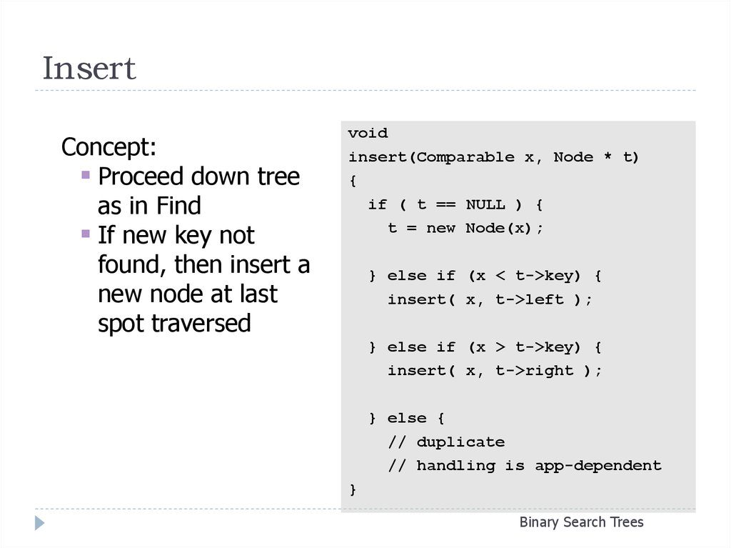
15. Insert

Concept:
Proceed down tree
as in Find
If new key not
found, then insert a
new node at last
spot traversed
void
insert(Comparable x, Node * t)
{
if ( t == NULL ) {
t = new Node(x);
} else if (x < t->key) {
insert( x, t->left );
} else if (x > t->key) {
insert( x, t->right );
} else {
// duplicate
// handling is app-dependent
}
Binary Search Trees

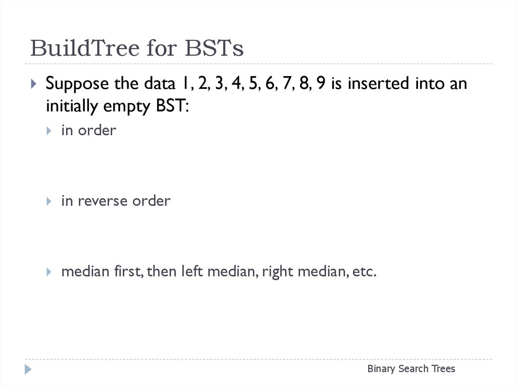
16. BuildTree for BSTs

Suppose the data 1, 2, 3, 4, 5, 6, 7, 8, 9 is inserted into an
initially empty BST:
in order
in reverse order
median first, then left median, right median, etc.
Binary Search Trees

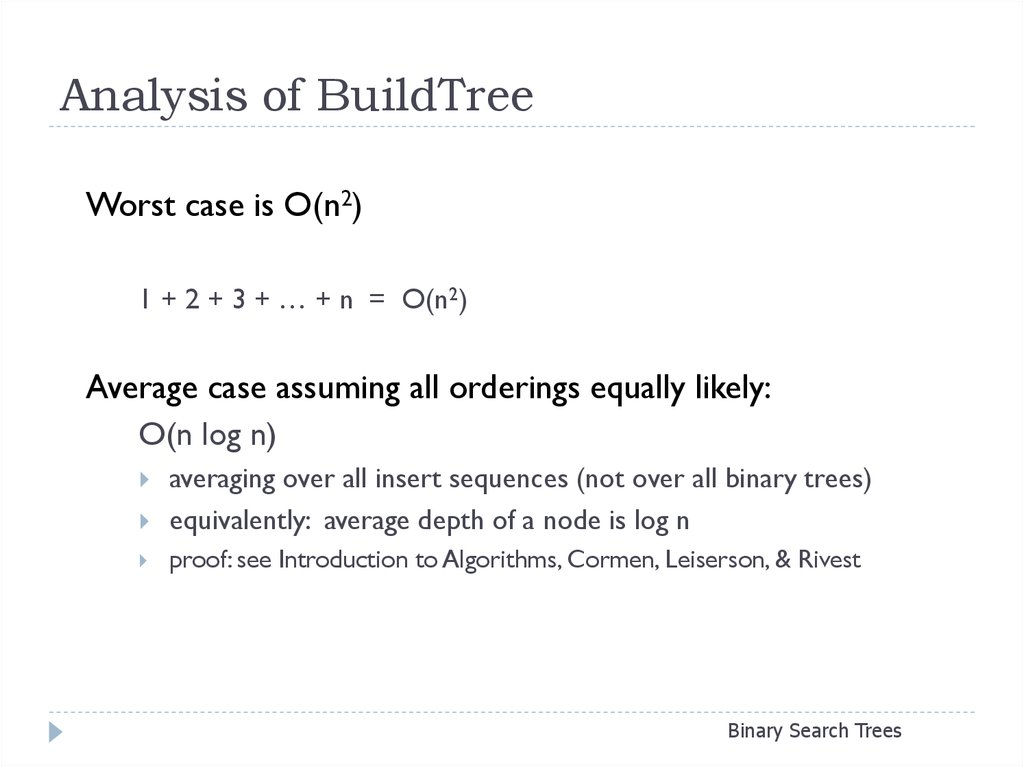
17. Analysis of BuildTree

Worst case is O(n2)
1 + 2 + 3 + … + n = O(n2)
Average case assuming all orderings equally likely:
O(n log n)
averaging over all insert sequences (not over all binary trees)
equivalently: average depth of a node is log n
proof: see Introduction to Algorithms, Cormen, Leiserson, & Rivest
Binary Search Trees

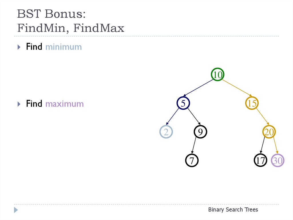
18. BST Bonus: FindMin, FindMax

Find minimum
10
Find maximum
5
15
2
9
7
20
17 30
Binary Search Trees

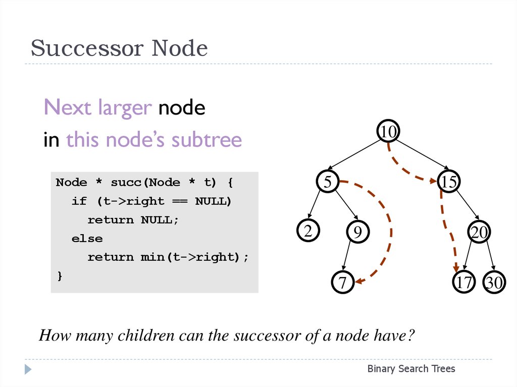
19. Successor Node

Next larger node
in this node’s subtree
Node * succ(Node * t) {
if (t->right == NULL)
return NULL;
else
return min(t->right);
}
10
5
15
2
9
20
17 30
7
How many children can the successor of a node have?
Binary Search Trees

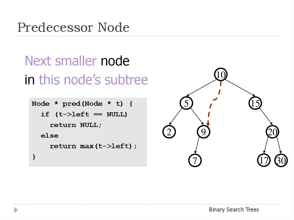
20. Predecessor Node

Next smaller node
in this node’s subtree
Node * pred(Node * t) {
if (t->left == NULL)
return NULL;
else
return max(t->left);
}
10
5
15
2
9
7
20
17 30
Binary Search Trees

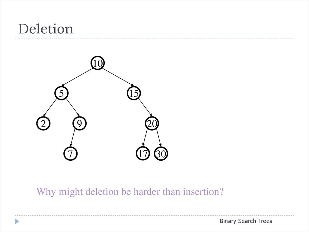
21. Deletion

10
5
15
2
9
7
20
17 30
Why might deletion be harder than insertion?
Binary Search Trees

22. Lazy Deletion

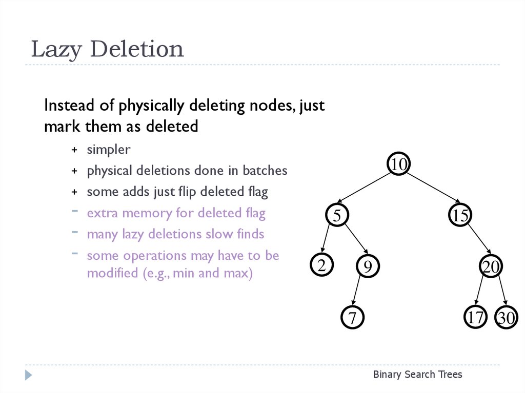
Instead of physically deleting nodes, just
mark them as deleted
+
+
+
-
simpler
physical deletions done in batches
some adds just flip deleted flag
extra memory for deleted flag
many lazy deletions slow finds
some operations may have to be
modified (e.g., min and max)
10
5
15
2
9
20
17 30
7
Binary Search Trees

23. Lazy Deletion

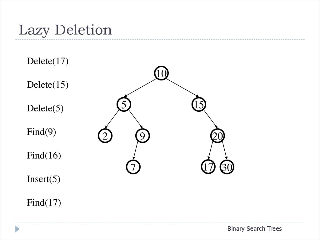
Delete(17)
10
Delete(15)
5
Delete(5)
Find(9)
15
2
9
20
Find(16)
7
17 30
Insert(5)
Find(17)
Binary Search Trees

24. Deletion - Leaf Case

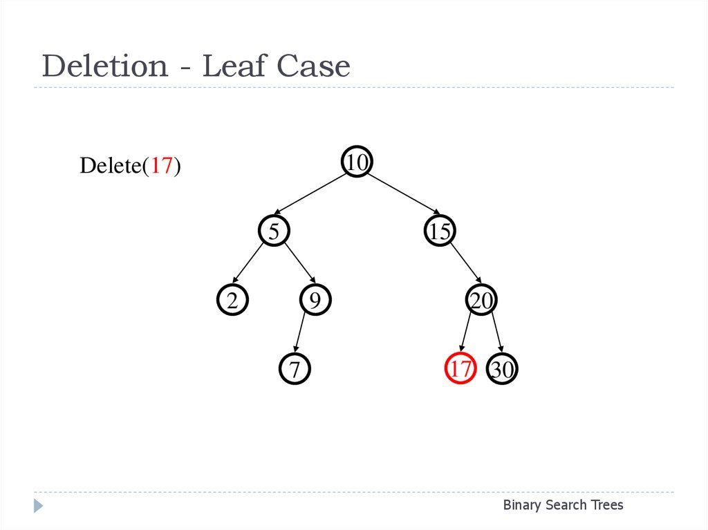
10
Delete(17)
5
15
2
9
7
20
17 30
Binary Search Trees

25. Deletion - One Child Case

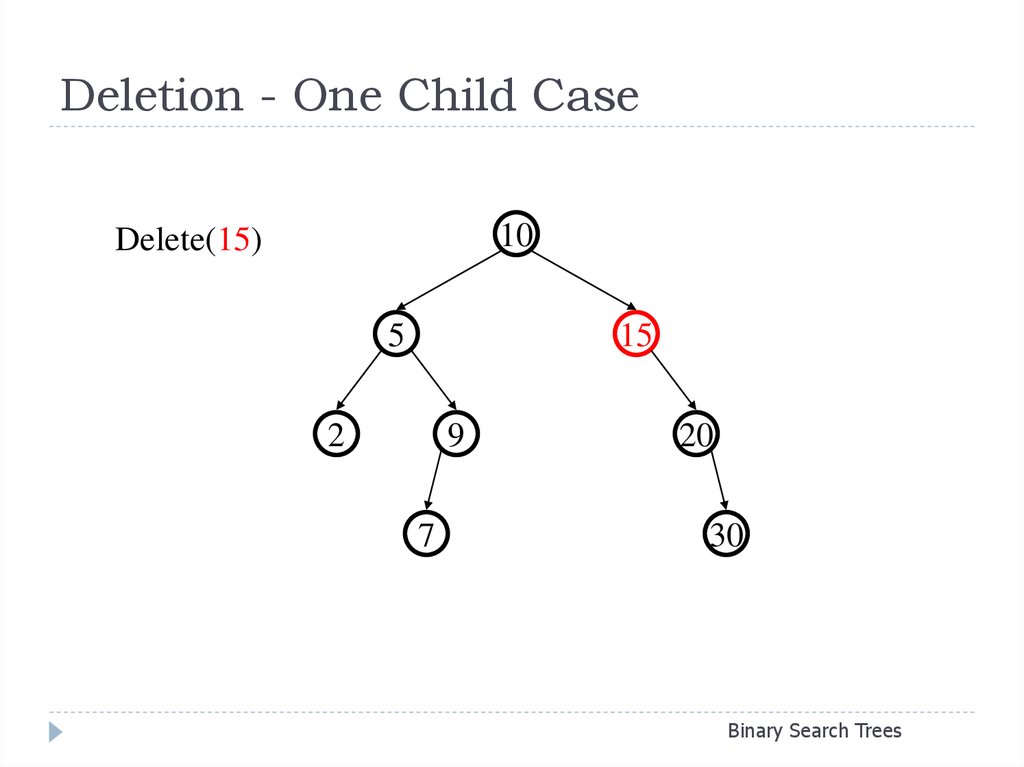
10
Delete(15)
5
15
2
9
7
20
30
Binary Search Trees

26. Deletion - Two Child Case

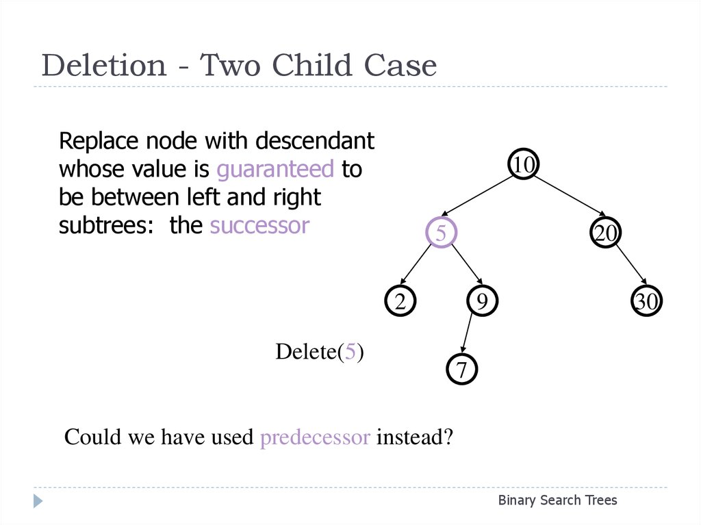
Replace node with descendant
whose value is guaranteed to
be between left and right
subtrees: the successor
10
5
20
2
Delete(5)
9
30
7
Could we have used predecessor instead?
Binary Search Trees

27. Delete Code

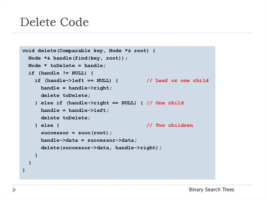
void delete(Comparable key, Node *& root) {
Node *& handle(find(key, root));
Node * toDelete = handle;
if (handle != NULL) {
if (handle->left == NULL) {
// Leaf or one child
handle = handle->right;
delete toDelete;
} else if (handle->right == NULL) { // One child
handle = handle->left;
delete toDelete;
} else {
// Two children
successor = succ(root);
handle->data = successor->data;
delete(successor->data, handle->right);
}
}
}
Binary Search Trees

28. Thinking about Binary Search Trees

Observations
Each operation views two new elements at a time
Elements (even siblings) may be scattered in memory
Binary search trees are fast if they’re shallow
Realities
For large data sets, disk accesses dominate runtime
Some deep and some shallow BSTs exist for any data
Binary Search Trees

29. Beauty is Only (log n) Deep

Beauty is Only (log n) Deep
Binary Search Trees are fast if they’re shallow:
perfectly complete
complete – possibly missing some “fringe” (leaves)
any other good cases?
What matters?
Problems occur when one branch is much longer than another
i.e. when tree is out of balance
Binary Search Trees

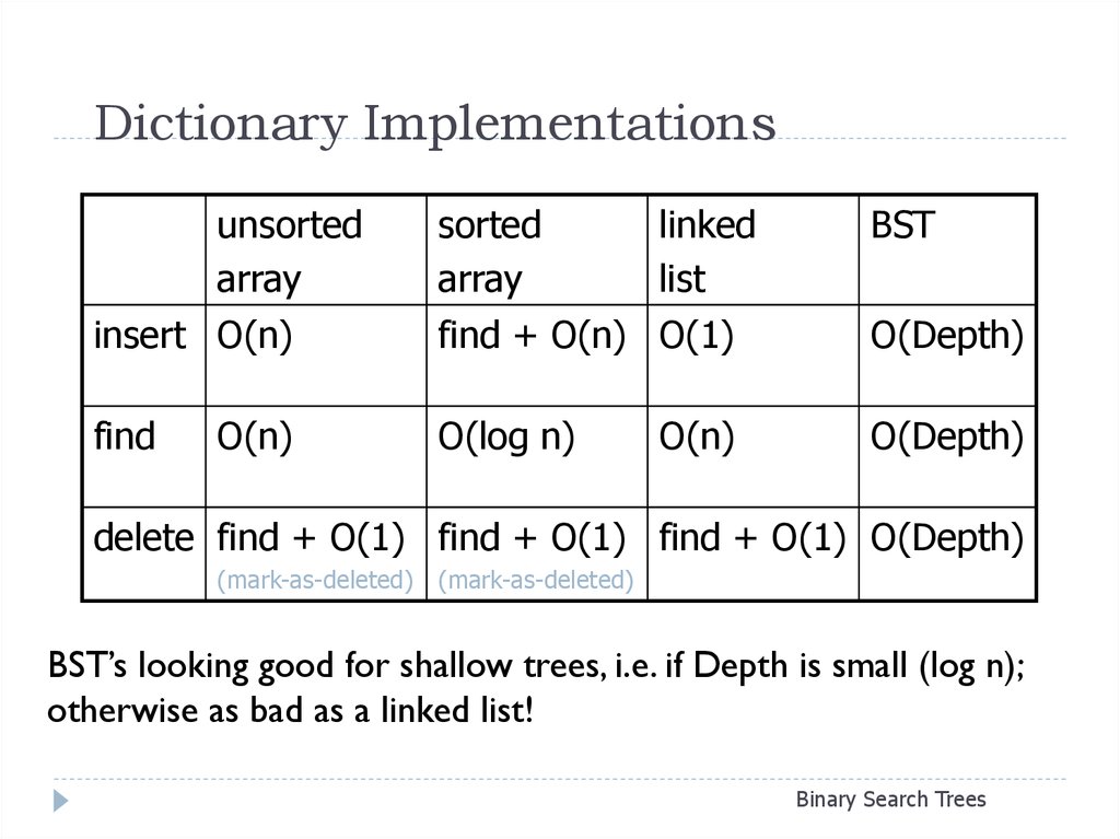
30. Dictionary Implementations

unsorted
array
insert O(n)
sorted
linked
array
list
find + O(n) O(1)
BST
find
O(log n)
O(Depth)
O(n)
O(n)
O(Depth)
delete find + O(1) find + O(1) find + O(1) O(Depth)
(mark-as-deleted) (mark-as-deleted)
BST’s looking good for shallow trees, i.e. if Depth is small (log n);
otherwise as bad as a linked list!
Binary Search Trees

31. Digression: Tail Recursion

Tail recursion: when the tail (final operation) of a function
recursively calls the function
Why is tail recursion especially bad with a linked list?
Why might it be a lot better with a tree? Why might it
not?
Binary Search Trees

32. Making Trees Efficient: Possible Solutions

Keep BSTs shallow by maintaining “balance”
AVL
trees
… also exploit most-recently-used (mru) info
Splay
trees
Reduce disk access by increasing branching factor
B-trees
Binary Search Trees