Похожие презентации:
Introduction to artificial intelligence А* Search
1. Introduction to Artificial Intelligence A* Search
Ruth BergmanFall 2004
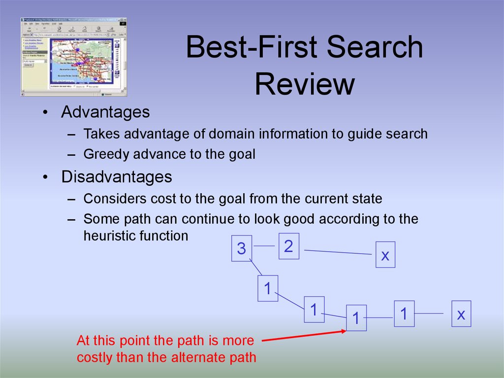
2. Best-First Search Review
• Advantages– Takes advantage of domain information to guide search
– Greedy advance to the goal
• Disadvantages
– Considers cost to the goal from the current state
– Some path can continue to look good according to the
heuristic function
2
3
x
1
1
At this point the path is more
costly than the alternate path
1
1
x
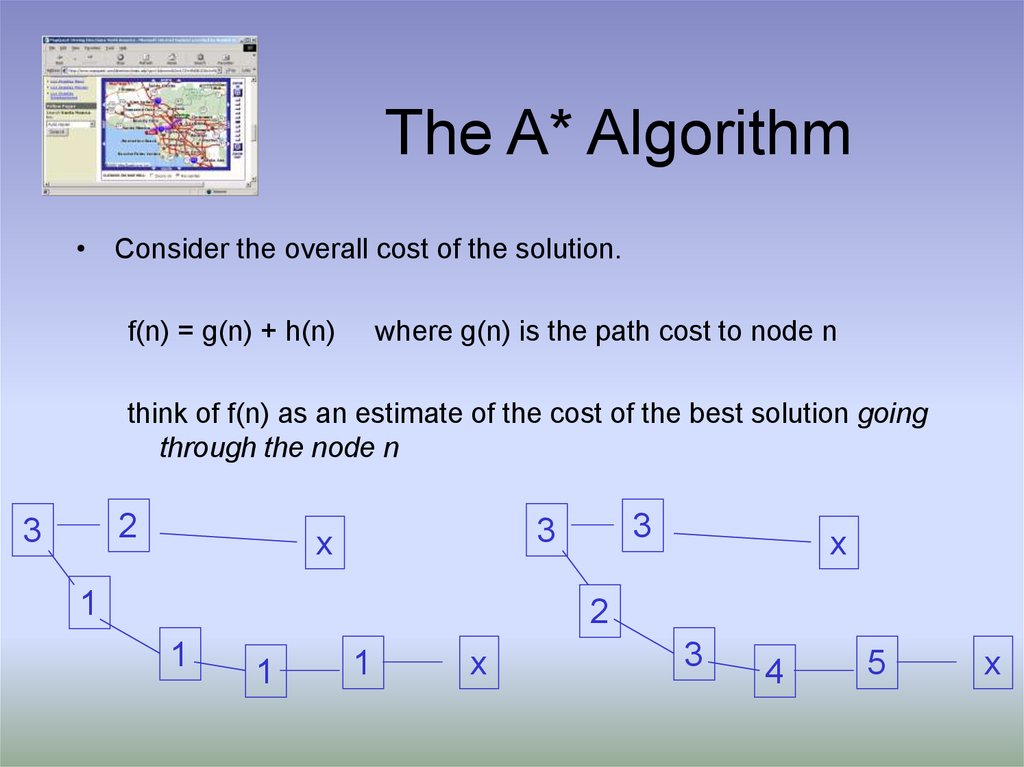
3. The A* Algorithm
• Consider the overall cost of the solution.f(n) = g(n) + h(n)
where g(n) is the path cost to node n
think of f(n) as an estimate of the cost of the best solution going
through the node n
2
3
3
3
x
1
x
2
1
1
1
x
3
4
5
x
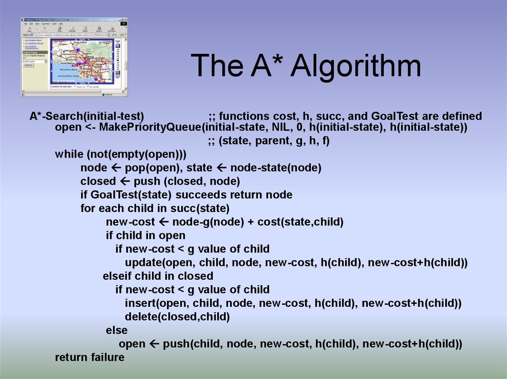
4. The A* Algorithm
A*-Search(initial-test);; functions cost, h, succ, and GoalTest are defined
open <- MakePriorityQueue(initial-state, NIL, 0, h(initial-state), h(initial-state))
;; (state, parent, g, h, f)
while (not(empty(open)))
node pop(open), state node-state(node)
closed push (closed, node)
if GoalTest(state) succeeds return node
for each child in succ(state)
new-cost node-g(node) + cost(state,child)
if child in open
if new-cost < g value of child
update(open, child, node, new-cost, h(child), new-cost+h(child))
elseif child in closed
if new-cost < g value of child
insert(open, child, node, new-cost, h(child), new-cost+h(child))
delete(closed,child)
else
open push(child, node, new-cost, h(child), new-cost+h(child))
return failure
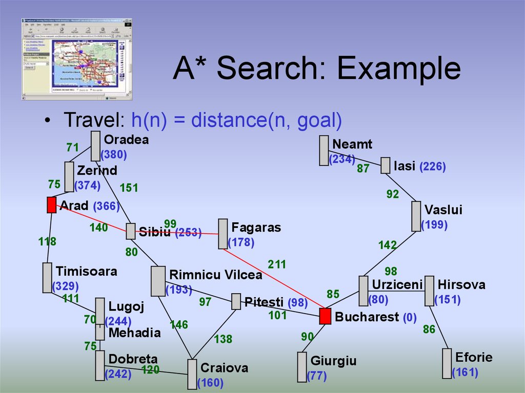
5. A* Search: Example
• Travel: h(n) = distance(n, goal)Oradea
71
Neamt
(380)
(234)
Zerind
75
(374)
Iasi (226)
87
151
92
Arad (366)
Vaslui
99
140
118
(178)
80
Timisoara
(329)
111
(199)
Fagaras
Sibiu (253)
Rimnicu Vilcea
142
211
98
(193)
70 (244)
Mehadia
75
Dobreta
(242) 120
Pitesti (98)
97
Lugoj
85
101
146
138
Craiova
(160)
Urziceni
(80)
Hirsova
(151)
Bucharest (0)
90
Giurgiu
(77)
86
Eforie
(161)
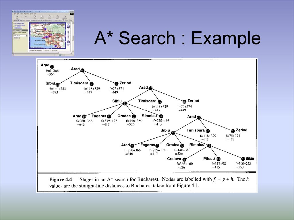
6. A* Search : Example
7. Admissible Heuristics
• we also require h be admissible:– a heuristic h is admissible if h(n) < h*(n) for all nodes n,
– where h* is the actual cost of the optimal path from n to the
goal
• Examples:
– travel distance straight line distance must be shorter than
actual travel path
– tiles out of place each move can reorder at most one tile
distance of each out of place tile from the correct place each
move moves a tile at most one place toward correct place
8. Optimality of A*
• Let us assume that f is non-decreasing along each path– if not, simply use parent’s value
– if that’s the case, we can think of A* as expanding f contours toward
the goal; better heuristics make this contour more “eccentric”
• Let G be an optimal goal state with path cost f*
• Let G2 be a suboptimal goal state with path cost g(G2) > f*.
–
–
–
–
–
–
–
suppose A* picks G2 before G (A* is not optimal)
suppose n is a leaf node on the path to G when G2 is chosen
if h is admissible, then f* >= f(n)
since n was not chosen, it must be the case that f(n) >= f(G2)
therefore f* >= f(G2), but since G2 is a goal, h(G2)=0, so f* >= g(G2)
But this is a contradiction --- G2 is a better goal node than G
Thus, our supposition is false and A* is optimal.
9. Completeness of A*
• Suppose there is a goal state G with path cost f*– Intuitively: since A* expands nodes in order of increasing f, it must
eventually expand node G
• If A* stops and fails
–
–
–
–
–
Prove by contradiction that this is impossible.
There exists a path from the initial state to the node state
Let n be the last node expanded along the solution path
n has at least one child, that child should be in the open nodes
A* does not stop until there are open list is empty (unless it finds a
goal state). Contradiction.
• A* is on an infinite path
– Recall that cost(s1,s2) > d
– Let n be the last node expanded along the solution path
– After f(n)/d the cumulative cost of the path becomes large enough
that A* will expand n. Contradiction.
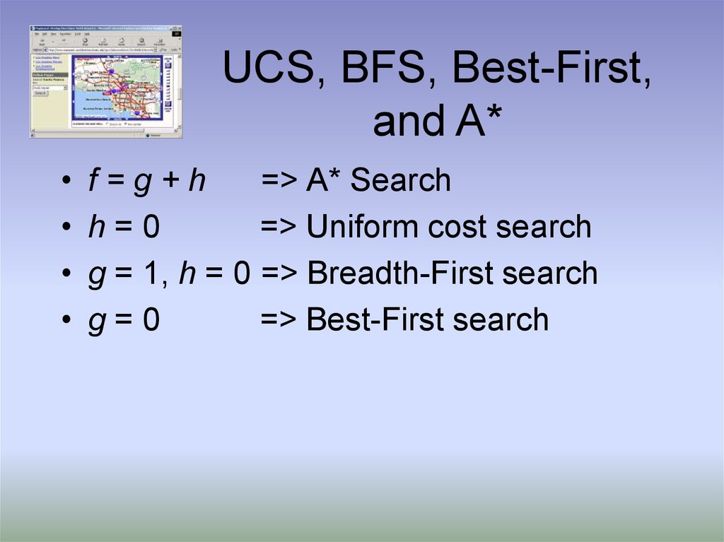
10. UCS, BFS, Best-First, and A*
f=g+h
=> A* Search
h=0
=> Uniform cost search
g = 1, h = 0 => Breadth-First search
g=0
=> Best-First search
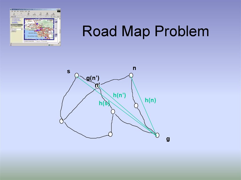
11. Road Map Problem
ns
g(n’)
n’
h(n’)
h(s)
h(n)
g
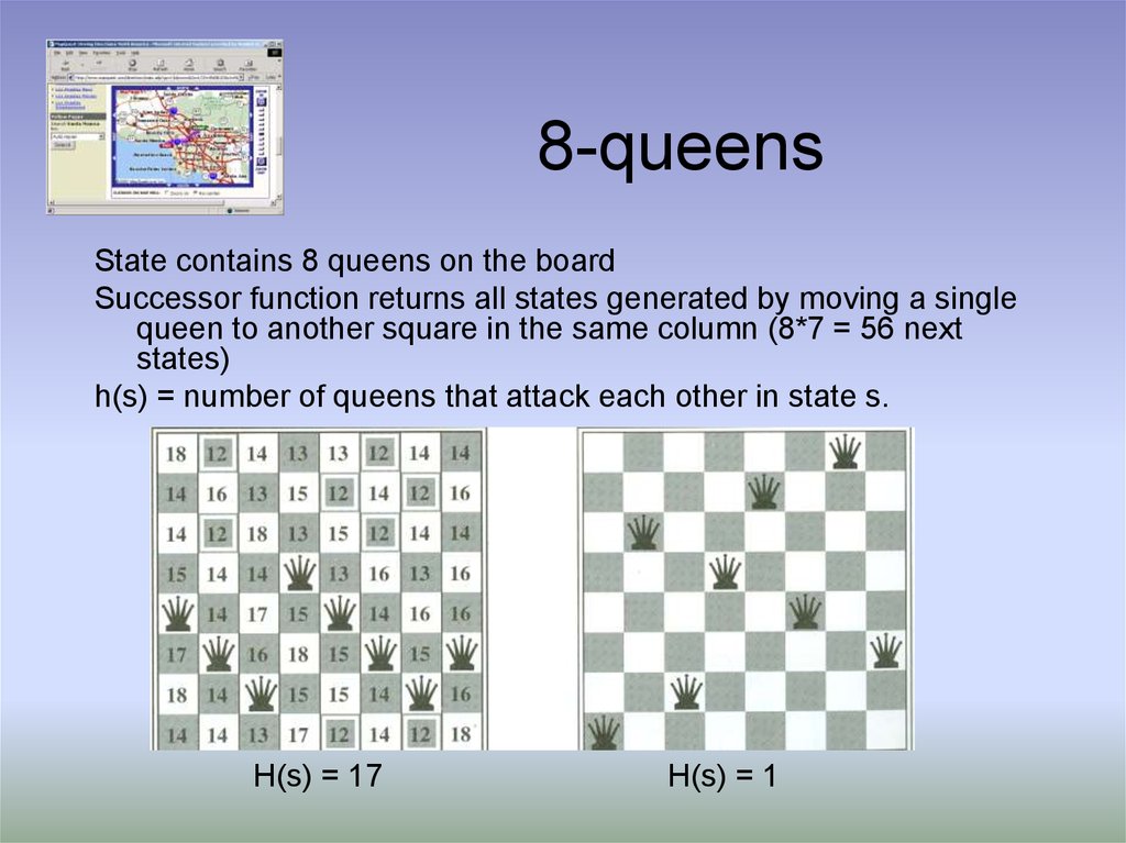
12. 8-queens
State contains 8 queens on the boardSuccessor function returns all states generated by moving a single
queen to another square in the same column (8*7 = 56 next
states)
h(s) = number of queens that attack each other in state s.
H(s) = 17
H(s) = 1
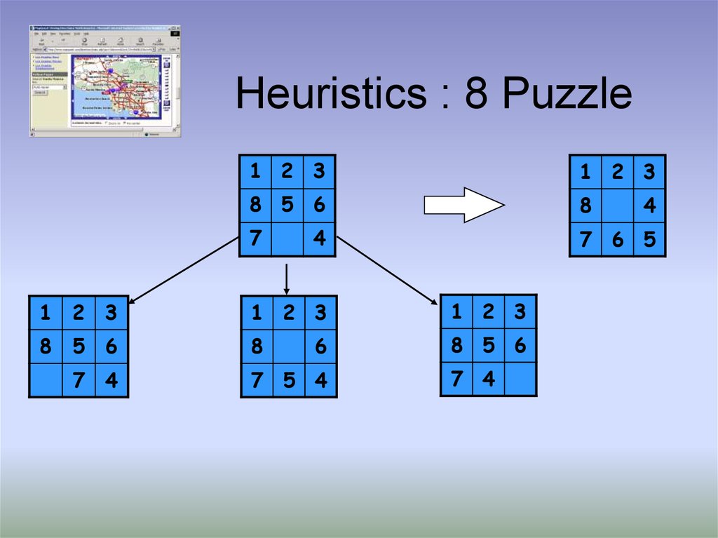
13. Heuristics : 8 Puzzle
1 2 31 2 3
8 5 6
8
7
7 6 5
4
1
2
3
1 2 3
1 2 3
8
5
6
8
8 5 6
7
4
7 5 4
6
7 4
4
14. 8 Puzzle
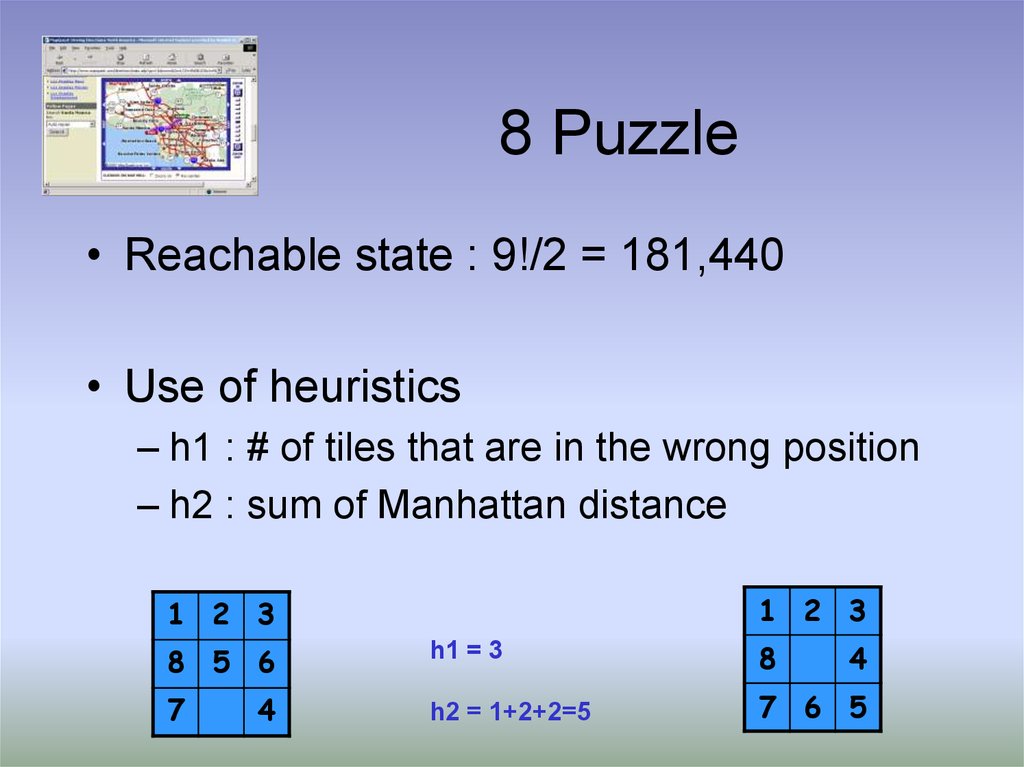
• Reachable state : 9!/2 = 181,440• Use of heuristics
– h1 : # of tiles that are in the wrong position
– h2 : sum of Manhattan distance
1 2 3
1 2 3
8 5 6
h1 = 3
8
7
h2 = 1+2+2=5
7 6 5
4
4
15. Effect of Heuristic Accuracy on Performance
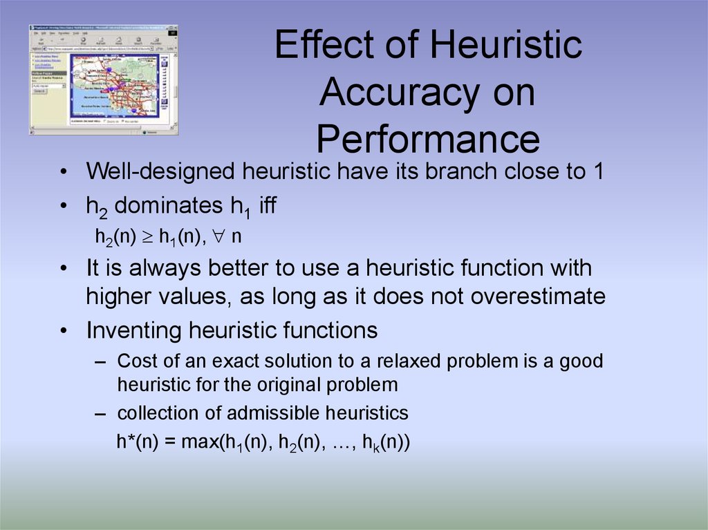
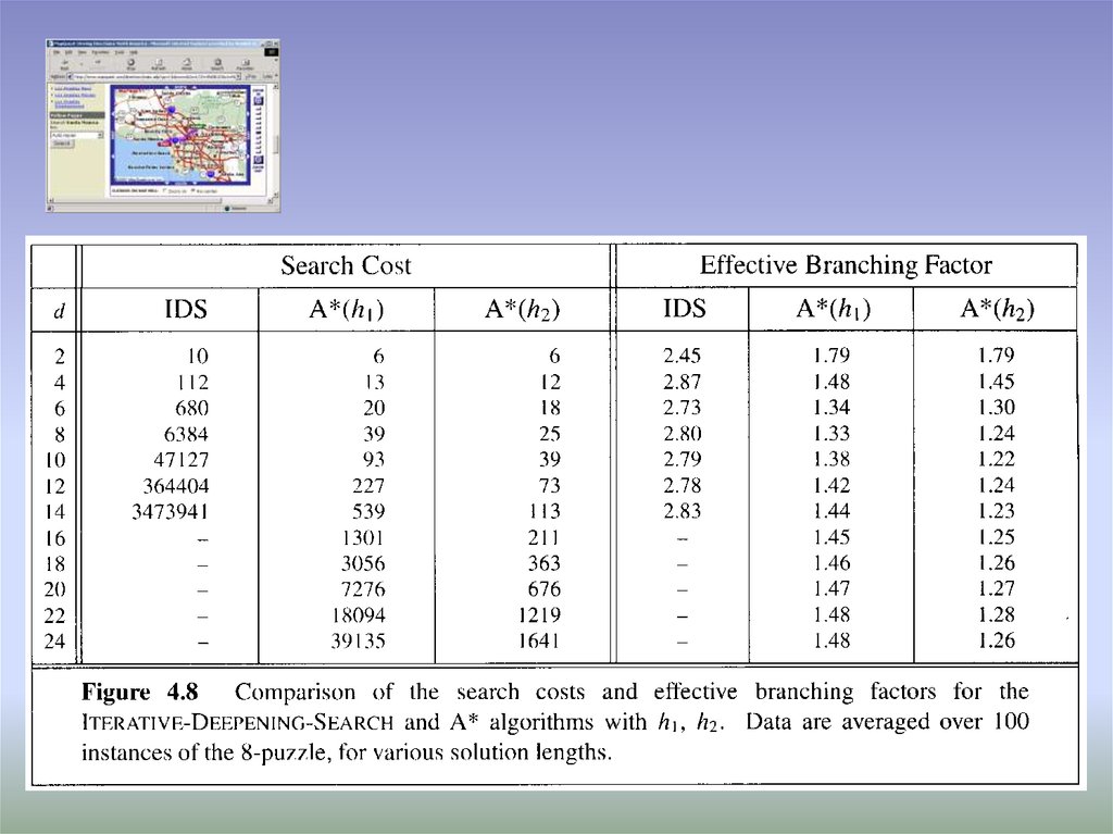
• Well-designed heuristic have its branch close to 1• h2 dominates h1 iff
h2(n) h1(n), n
• It is always better to use a heuristic function with
higher values, as long as it does not overestimate
• Inventing heuristic functions
– Cost of an exact solution to a relaxed problem is a good
heuristic for the original problem
– collection of admissible heuristics
h*(n) = max(h1(n), h2(n), …, hk(n))
16.
17. A* summary
• Completeness– provided finite branching factor and finite cost per operator
• Optimality
– provided we use an admissible heuristic
• Time complexity
– worst case is still O(bd) in some special cases we can do
better for a given heuristic
• Space complexity
– worst case is still O(bd)
18. Relax Optimality
• Goals:– Minimizing search cost
– Satisficing solution, i.e. bounded error in the
solution
f(s) = (1-w) g(s) + w h(s)
–
–
–
–
g can be thought of as the breadth first component
w = 1 => Best-First search
w = .5 => A* search
w = 0 => Uniform search
19. Iterative Deepening A*
• Goals– A storage efficient algorithm that we can use in practice
– Still complete and optimal
• Modification of A*
– use f-cost limit as depth bound
– increase threshold as minimum of f(.) of previous cycle
• Each iteration expands all nodes inside the contour
for current f-cost
• same order of node expansion
20. IDA* Algorithm
IDA* (state,h) returns solutionf-limit <- h(state)
loop do
solution, f-limit DFS-Contour(state, f-limit)
if solution is non-null return solution
if f-limit = return failure
end
DFS-Contour (node,f-limit) returns solution
if f (node) > f-limit return null, f(node)
if GoalTest(node) return node, f-limit
next-f
for each node s in succ(node) do
solution, new-f DFS-Contour(s, f-limit)
if solution is non-null return solution, f-limit
next-f Min(next-f, new-f)
end
return null, next-f
21. IDA* Properties
• Complete:– if shortest path fits into memory
• Optimal:
– if shortest optimal path fits into memory
• Time Complexity: O(b2d)
• Space Complexity: O(bd)
22. Mapquest
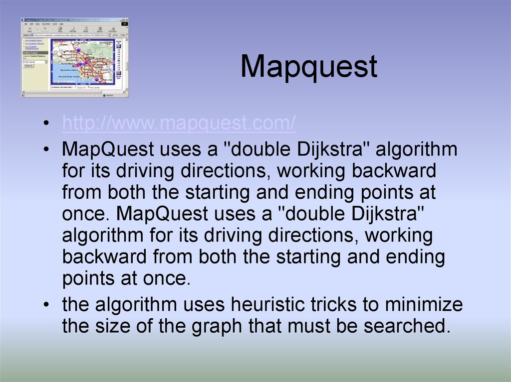
• http://www.mapquest.com/• MapQuest uses a "double Dijkstra" algorithm
for its driving directions, working backward
from both the starting and ending points at
once. MapQuest uses a "double Dijkstra"
algorithm for its driving directions, working
backward from both the starting and ending
points at once.
• the algorithm uses heuristic tricks to minimize
the size of the graph that must be searched.

 Программирование


