System models

1. AUTOMATICS and AUTOMATIC CONTROL

LECTURE 2
dr inż. Adam Kurnicki
Automation and Metrology Department
Room no 210A

2.

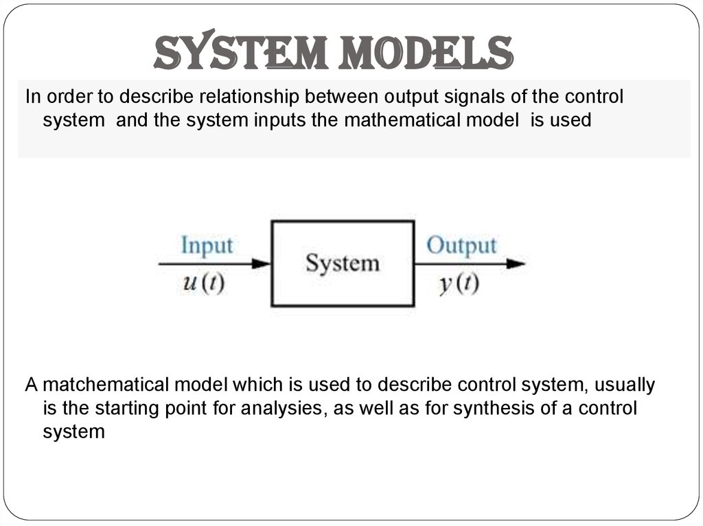
System models
In order to describe relationship between output signals of the control
system and the system inputs the mathematical model is used
A matchematical model which is used to describe control system, usually
is the starting point for analysies, as well as for synthesis of a control
system

3.

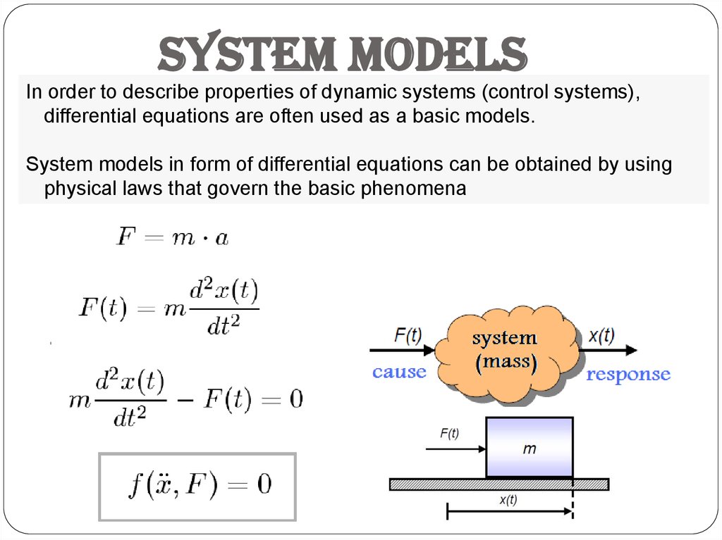
System models
In order to describe properties of dynamic systems (control systems),
differential equations are often used as a basic models.
System models in form of differential equations can be obtained by using
physical laws that govern the basic phenomena

4.

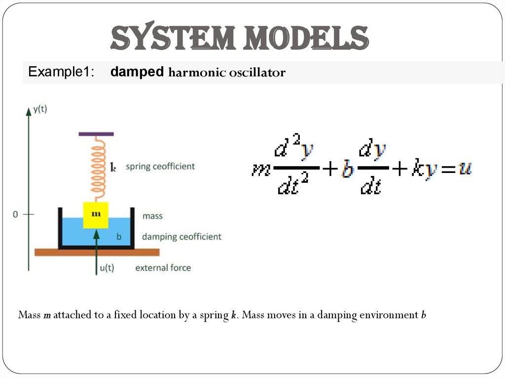
System models
Example1:
damped harmonic oscillator
Mass m attached to a fixed location by a spring k. Mass moves in a damping environment b

5.

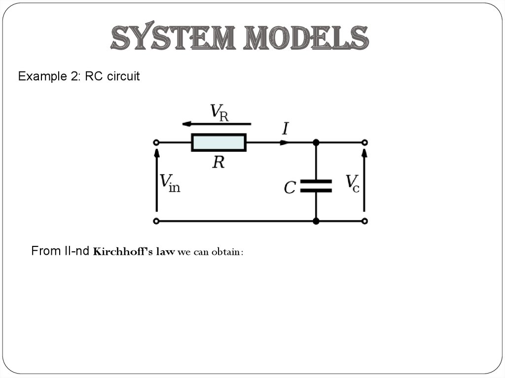
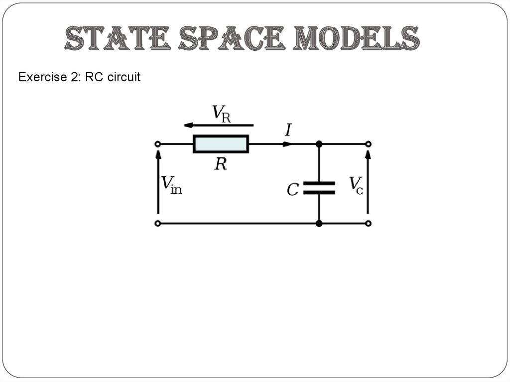
System models
Example 2: RC circuit
From II-nd Kirchhoff's law we can obtain:

6.

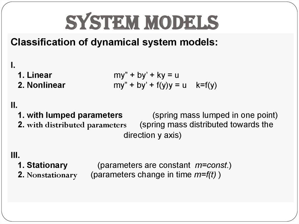
System models
Classification of dynamical system models:
I.
1. Linear
2. Nonlinear
my” + by’ + ky = u
my” + by’ + f(y)y = u
k=f(y)
II.
1. with lumped parameters
(spring mass lumped in one point)
2. with distributed parameters
(spring mass distributed towards the
direction y axis)
III.
1. Stationary
2. Nonstationary
(parameters are constant m=const.)
(parameters change in time m=f(t) )

7.

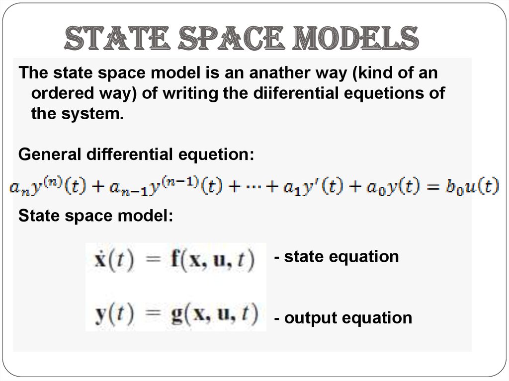
State space models
The state space model is an anather way (kind of an
ordered way) of writing the diiferential equetions of
the system.
General differential equetion:
State space model:
- state equation
- output equation

8.

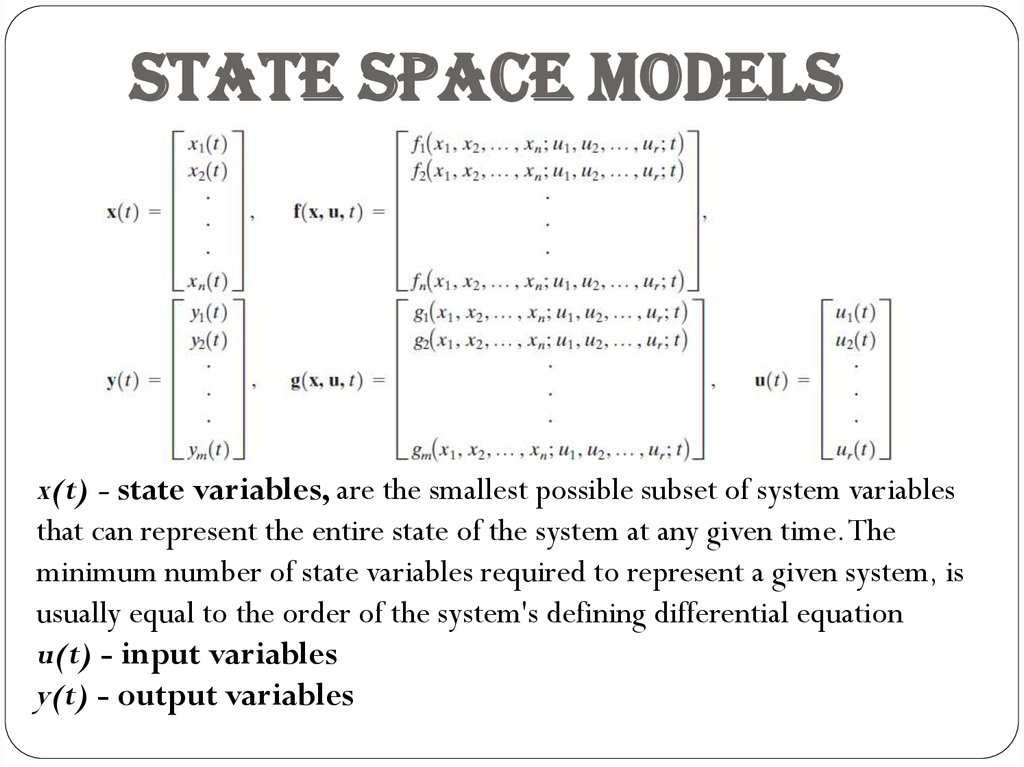
State space models
x(t) - state variables, are the smallest possible subset of system variables
that can represent the entire state of the system at any given time. The
minimum number of state variables required to represent a given system, is
usually equal to the order of the system's defining differential equation
u(t) - input variables
y(t) - output variables

9.

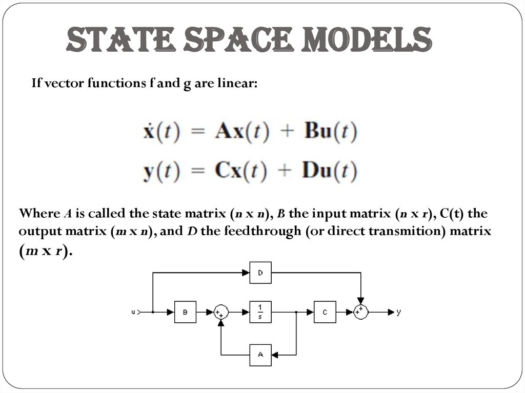
State space models
If vector functions f and g are linear:
Where A is called the state matrix (n x n), B the input matrix (n x r), C(t) the
output matrix (m x n), and D the feedthrough (or direct transmition) matrix
(m x r).

10.

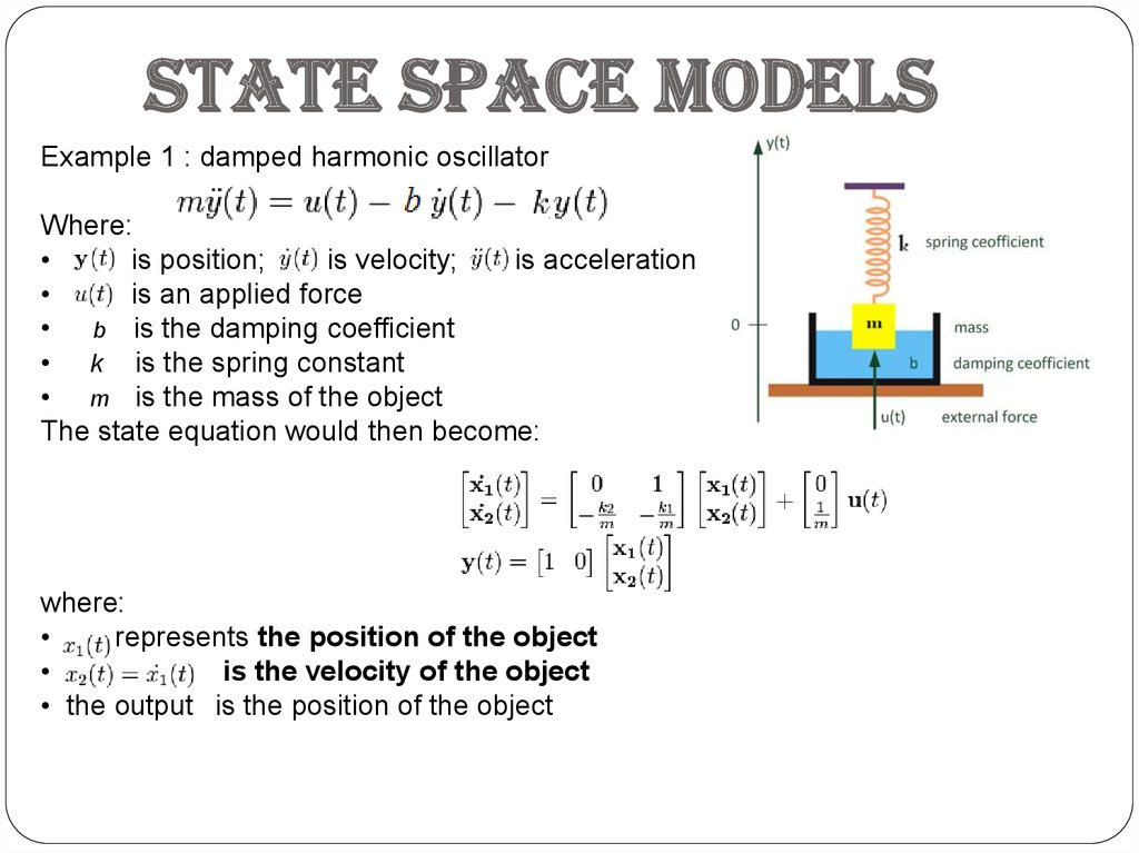
State space models
Example 1 : damped harmonic oscillator
Where:
is position;
is velocity;
is acceleration
is an applied force
• b is the damping coefficient
• k is the spring constant
• m is the mass of the object
The state equation would then become:
where:
represents the position of the object
is the velocity of the object
• the output is the position of the object

11.

State space models
Exercise 2: RC circuit

12.

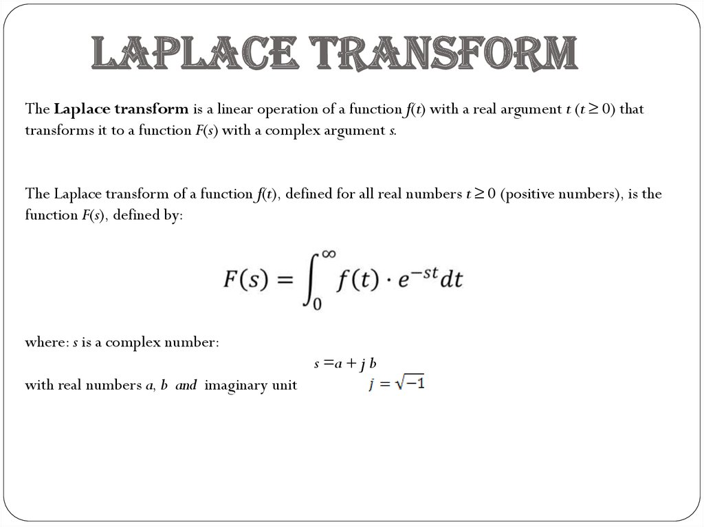
Laplace Transform
The Laplace transform is a linear operation of a function f(t) with a real argument t (t ≥ 0) that
transforms it to a function F(s) with a complex argument s.
The Laplace transform of a function f(t), defined for all real numbers t ≥ 0 (positive numbers), is the
function F(s), defined by:
where: s is a complex number:
s =a + j b
with real numbers a, b and imaginary unit

13.

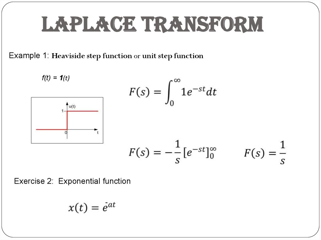
Laplace Transform
Example 1: Heaviside step function or unit step function
f(t) = 1(t)
Exercise 2: Exponential function
-

14.

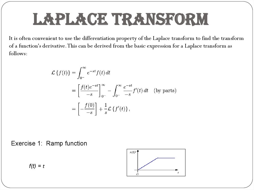
Laplace Transform
It is often convenient to use the differentiation property of the Laplace transform to find the transform
of a function's derivative. This can be derived from the basic expression for a Laplace transform as
follows:
Exercise 1: Ramp function
f(t) = t

15.

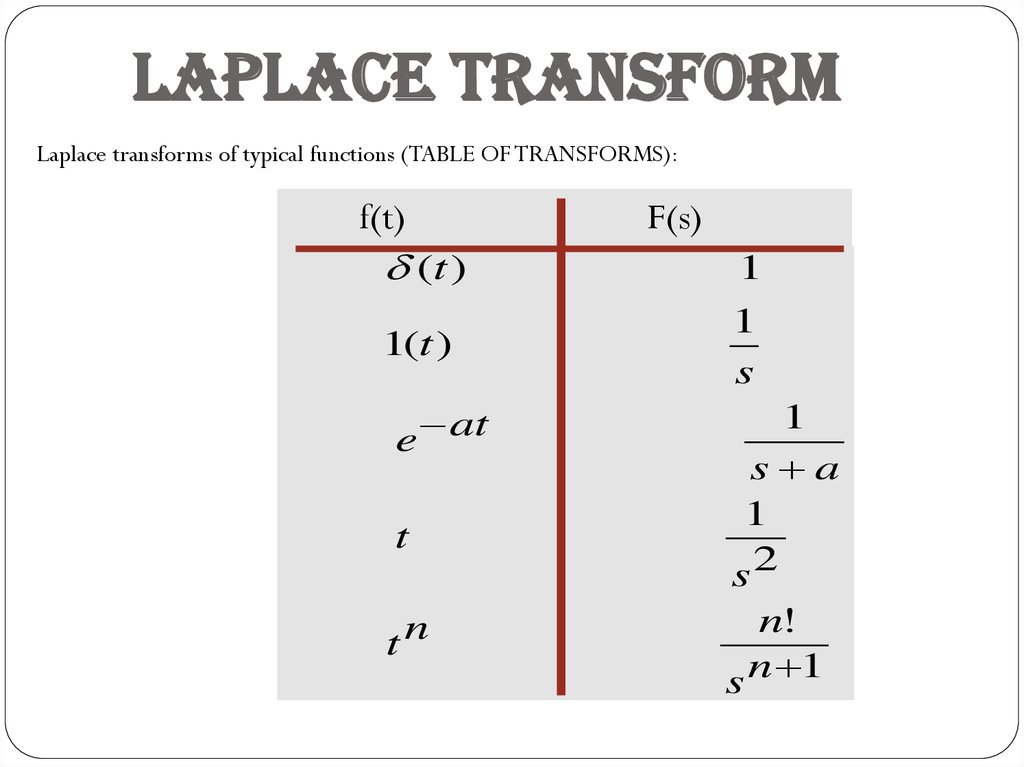
Laplace Transform
Laplace transforms of typical functions (TABLE OF TRANSFORMS):
f(t)
(t )
F(s)
1
1
1(t )
f (t )
F ( s)
s
____________________________________
1
at
e
s a
1
t
s2
tn
n!
s n 1

16.

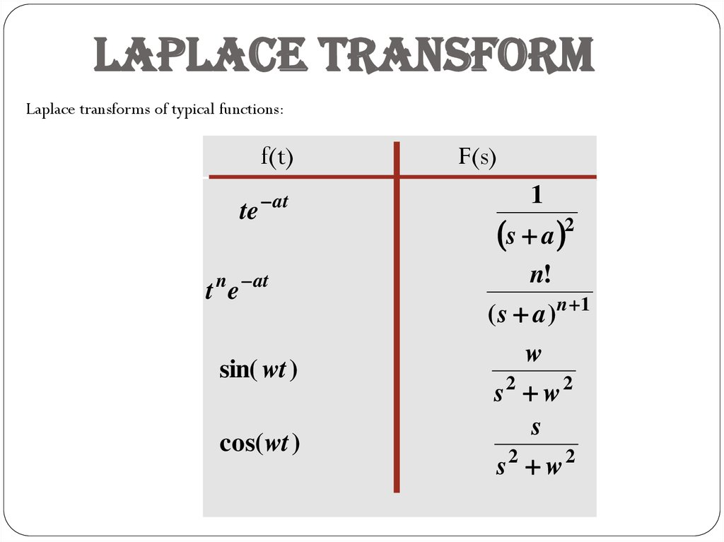
Laplace Transform
Laplace transforms of typical functions:
f(t)
te
at
n at
t e
sin( wt )
cos(wt )
F(s)
1
s a 2
n!
( s a )n 1
w
s2 w2
s
s2 w2

17.

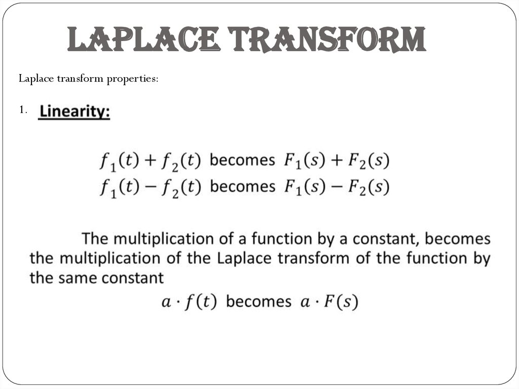
Laplace Transform
Laplace transform properties:
1.

18.

Laplace Transform
Laplace transform properties:
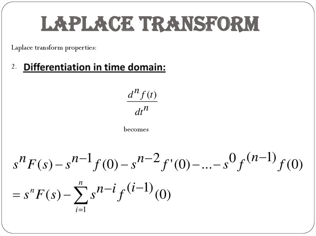
2.
d n f (t )
dt n
becomes
(n 1)
n
n
1
n
2
0
s F (s) s
f (0) s
f ' (0) ... s f
f (0)
n
s F ( s)
n
i 1
(i 1)
n
i
s
f
(0)

19.

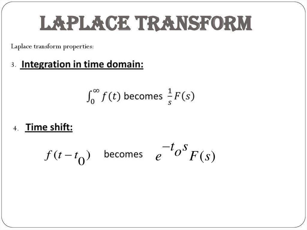
Laplace Transform
Laplace transform properties:
3.
4.
f (t t )
0
e
to s
F (s )

20.

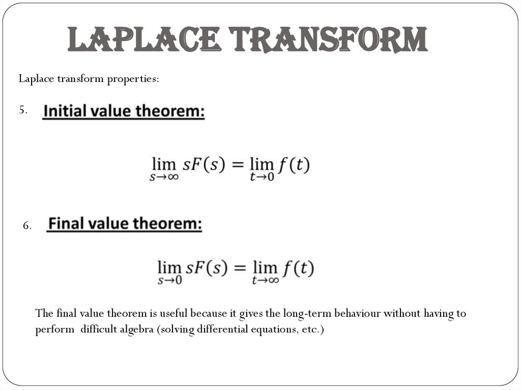
Laplace Transform
Laplace transform properties:
5.
6.
The final value theorem is useful because it gives the long-term behaviour without having to
perform difficult algebra (solving differential equations, etc.)

21.

Inverse Laplace Transform
The Inverse Laplace Transform is defined by:
1
L [ F ( s)] f (t )
1
2
j
F ( s )e
j
ts
ds
j
If the algebraic equation is solved in s, we can find the solution of
the differential equation using Inverse Laplace transform.
The most common procedure is to break the function F(s) in
fractions, calculate the inverse transforms in each, using
the transform table and add the analytical expressions for each
of them to find the function f(t) (partial fractions decomposition
or expansion)

22. TRANSFER FUNCTION

Transfer function is defined as the ratio of the Laplace
transform of the output signal to the Laplace transform of
the input signal under the assumption that all initial
conditions are zero)
Y ( s)
G( s)
U ( s)

23. TRANSFER FUNCTION

From general differential equetion:
a n y ( n ) (t ) a n 1 y ( n 1) (t ) ... a1 y ' (t ) a0 y (t ) bm u ( m ) (t ) bm 1u ( m 1) (t ) ... b1u ' (t ) b0 u (t )
we can obtain transfer function :
m 1
bm s bm 1 s ... b1 s b0
G( s)
a n s n a n 1 s n 1 ... a1 s a0
m

24. TRANSFER FUNCTION

Example1 : RC circuit

25. TRANSFER FUNCTION

Example2 : damped harmonic oscillator

26. TRANSFER FUNCTION

If we obtain the roots in the numerator and denominator of transfer function:
bm s m bm 1 s m 1 ... b1 s b0
G( s)
a n s n a n 1 s n 1 ... a1 s a0
we can change the standard form of transfer function to the form of ZERO-POLE:
z1, z2,… z3: zeros, numbers of s which makes the transfer function zero
p1, p2,… p3: poles, numbers of s which make the transfer function infinity
K is the gain
Zeros and poles could be complex numbers

27. TRANSFER FUNCTION AND STATE SPACE

We can transform State space model to transfer function by performing following operations:
Since the transfer function was previously defined as the ratio of the Laplace transform
of the output to the Laplace transform of the input when the initial conditions were
zero, we set x(0) in the previous equation to be zero. We operate and substitute and
then we have:
,I – unit matrix
and finally:

28. Model linearization

Control systems often works with small changes of input and output quantities around some
given steady state value. For this small changes the system can be described in an approximate
way by linear equation (differential equation)
• Static linearization
Taylor series expansion in steady state point:
because
:
⇒

29. Model linearization

• Static linearization example:
• Static linearization exercise:
Pendulum T=m*g*l*sin(x) (To,xo) = (0,0)

30. Model linearization

• Linearization of differential equation (dynamic linearization)
Taylor series expansion in steady state point
because
:
:

31. Model linearization

• Linearization of differential equation (dynamic linearization) example:
DC generator equation:

32. THANK YOU