Basics of time series forecasting. Lecture 9

1.

2.

LECTURE 9
BASICS OF TIME SERIES FORECASTING
Saidgozi Saydumarov
Sherzodbek Safarov
QM Module Leaders
[email protected]
[email protected]
Office hours: by appointment
Room IB 205
EXT: 546

3.

Lecture outline:
to estimate the change of a value over time and graph the
dynamics of the value
to apply the time series analysis to forecasting a value
to use the two forecasting models:
a)
Additive
b)
Multiplicative

4.

Components of time series graph
Trend –
the overall pattern of changes in a specific value over a
long period of time (or an overall movement of the
time series
graph).
Seasonal – regular patterns of variation over one year or less (or
repetitive movements of the time series graph).
Irregular – random changes that generally cannot be predicted (or
random movements of the time series graph for periods less than a
year).
Cyclical – variations above or below the trend line for periods of longer
than one year (or cyclical movements of the time series graph for periods
of longer than one year)

5.

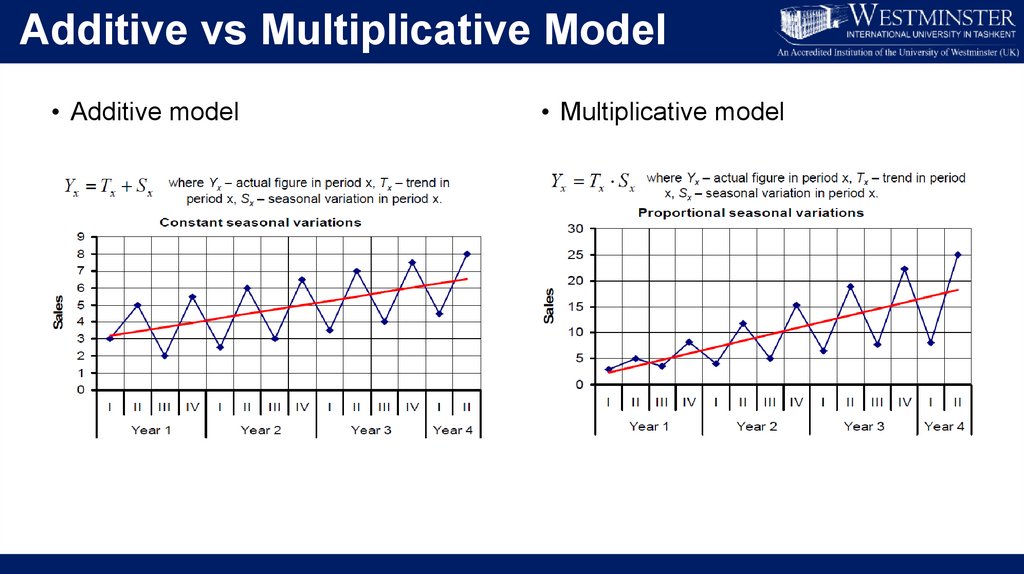
Additive vs Multiplicative Model
• Additive model
• Multiplicative model

6.

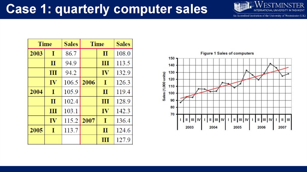
Case 1: quarterly computer sales

7.

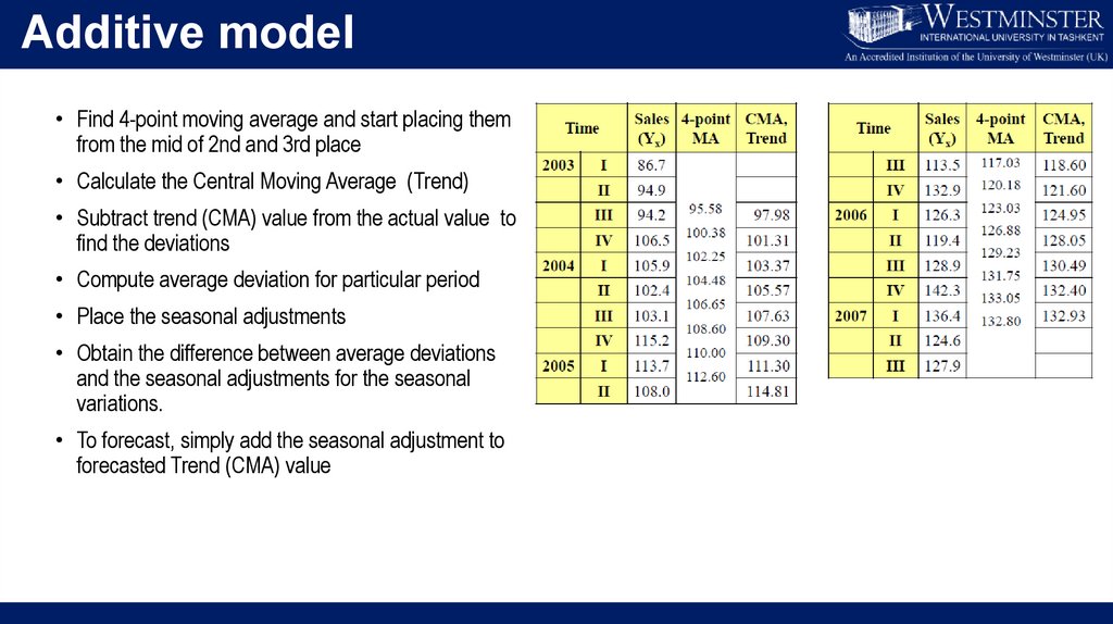
Additive model
• Find 4-point moving average and start placing them
from the mid of 2nd and 3rd place
• Calculate the Central Moving Average (Trend)
• Subtract trend (CMA) value from the actual value to
find the deviations
• Compute average deviation for particular period
• Place the seasonal adjustments
• Obtain the difference between average deviations
and the seasonal adjustments for the seasonal
variations.
• To forecast, simply add the seasonal adjustment to
forecasted Trend (CMA) value

8.

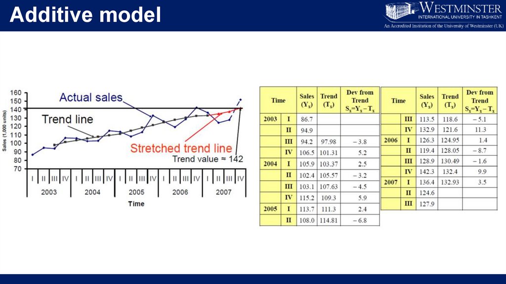
Additive model

9.

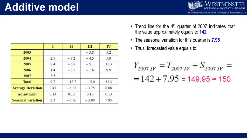
Additive model
• Trend line for the 4th quarter of 2007 indicates that
the value approximately equals to 142
• The seasonal variation for this quarter is 7.95
• Thus, forecasted value equals to

10.

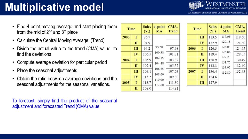
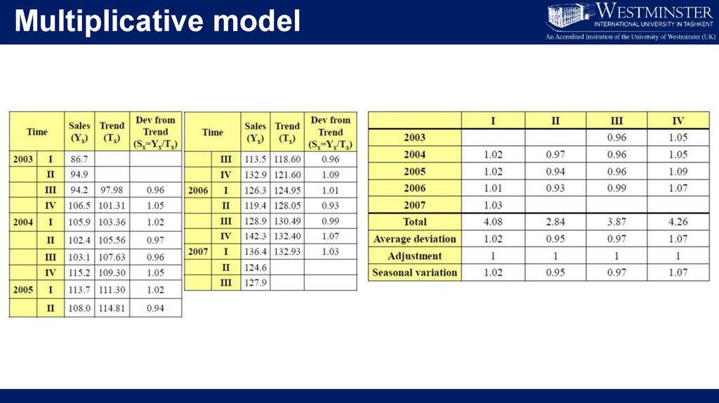
Multiplicative model
• Find 4-point moving average and start placing them
from the mid of 2nd and 3rd place
• Calculate the Central Moving Average (Trend)
• Divide the actual value to the trend (CMA) value to
find the deviations
• Compute average deviation for particular period
• Place the seasonal adjustments
• Obtain the ratio between average deviations and the
seasonal adjustments for the seasonal variations.
To forecast, simply find the product of the seasonal
adjustment and forecasted Trend (CMA) value

11.

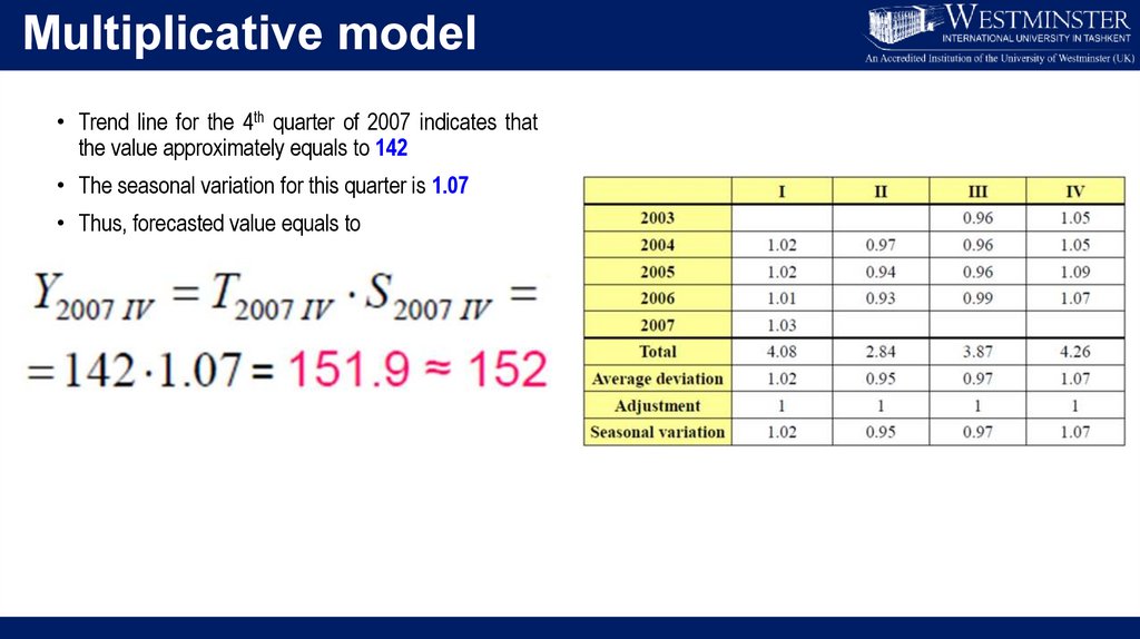
Multiplicative model

12.

Multiplicative model
• Trend line for the 4th quarter of 2007 indicates that
the value approximately equals to 142
• The seasonal variation for this quarter is 1.07
• Thus, forecasted value equals to

13.

Concluding remarks
Today, you learned
Graphical display of the change of a value over time
Time series analysis
Two time series models: additive and multiplicative
Forecasting future value with the suitable model

14.

Essential readings
Jon Curwin and Roger Slater. “Quantitative Methods for Business
Decisions,” Ch 17.