The Distribution of Molecules over Velocities Maxwell Distribution

1.

MEPhI General Physics
Lecture 09
The Distribution of Molecules
over Velocities
Maxwell Distribution

2.

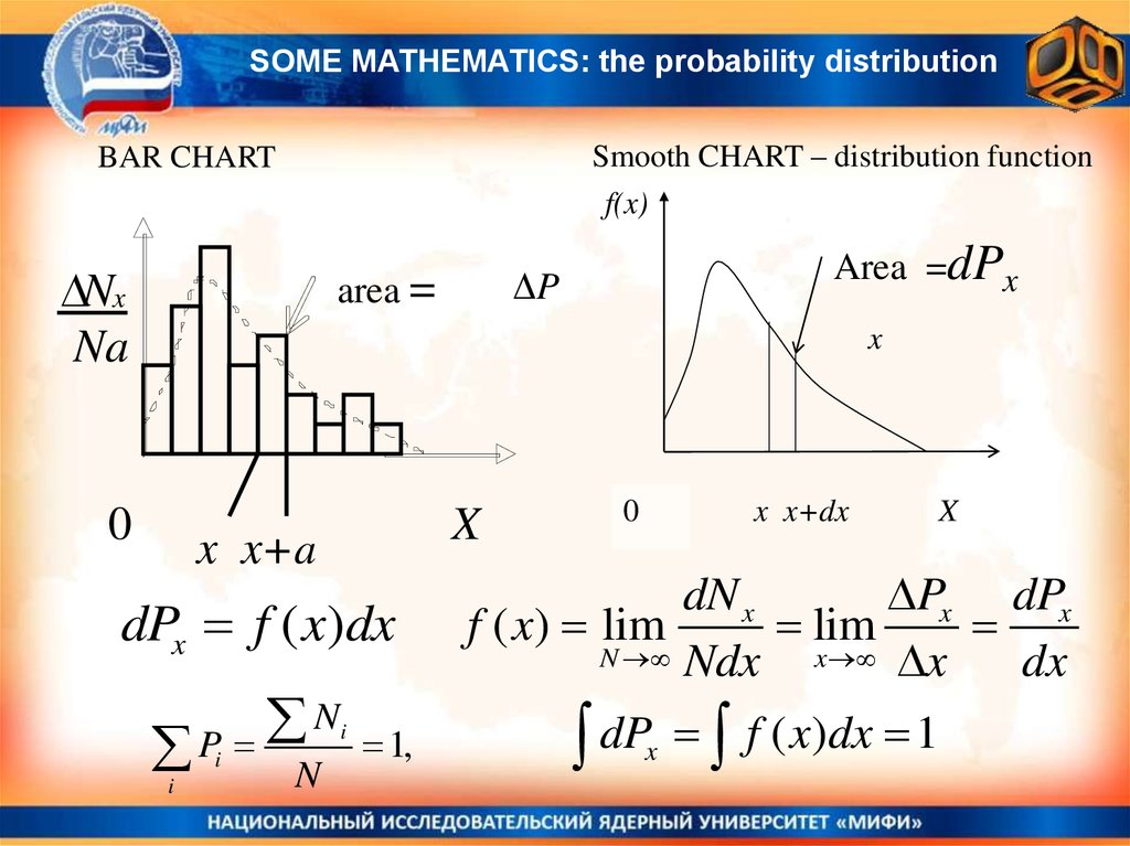
SOME MATHEMATICS: the probability distribution
Smooth CHART – distribution function
f(x)
BAR CHART
Nx
Na
Area =dPx
ΔP
area =
x
0
X
x x+a
dPx f ( x)dx
N
P
i
i
N
i
1,
0
x x+dx
X
dN x
Px dPx
f ( x) lim
lim
N Ndx
x x
dx
dP f ( x)dx 1
x

3.

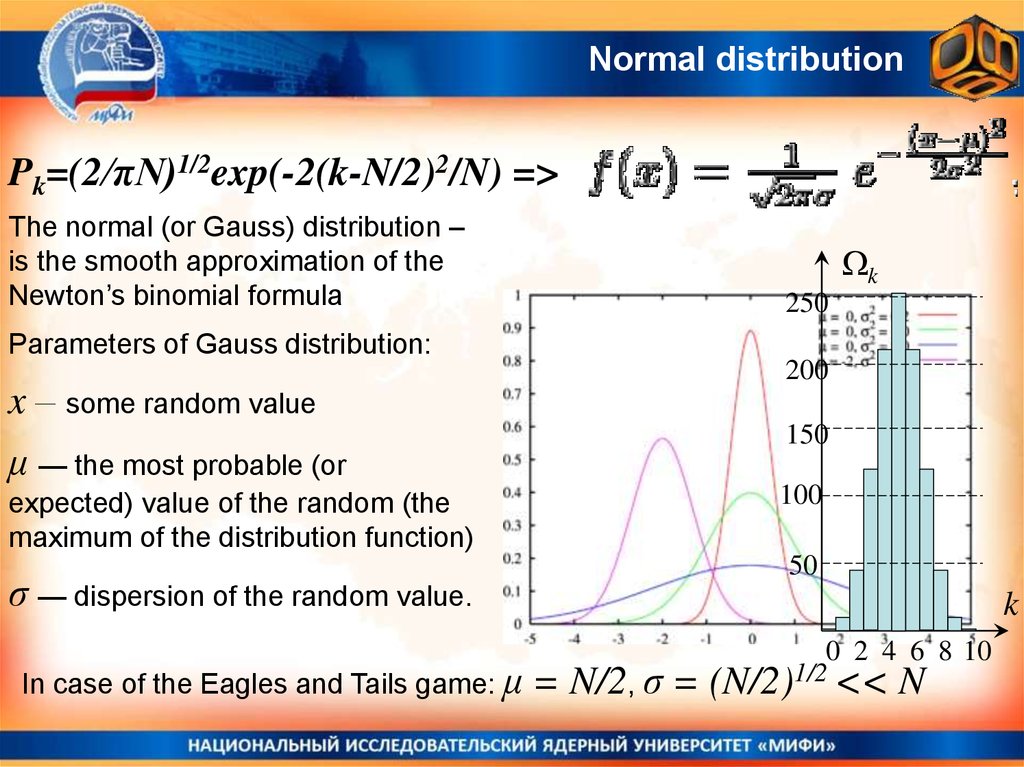
Normal distribution
Pk=(2/πN)1/2exp(-2(k-N/2)2/N) =>
The normal (or Gauss) distribution –
is the smooth approximation of the
Newton’s binomial formula
k
250
Parameters of Gauss distribution:
x – some random value
μ — the most probable (or
expected) value of the random (the
maximum of the distribution function)
σ — dispersion of the random value.
In case of the Eagles and Tails game: μ
200
150
100
50
k
0 2 4 6 8 10
= N/2, σ = (N/2)1/2 << N

4.

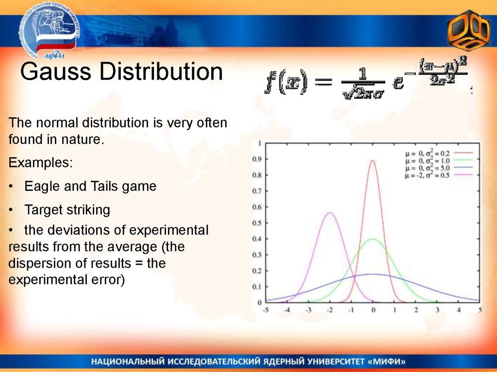
Gauss Distribution
The normal distribution is very often
found in nature.
Examples:
• Eagle and Tails game
• Target striking
• the deviations of experimental
results from the average (the
dispersion of results = the
experimental error)

5.

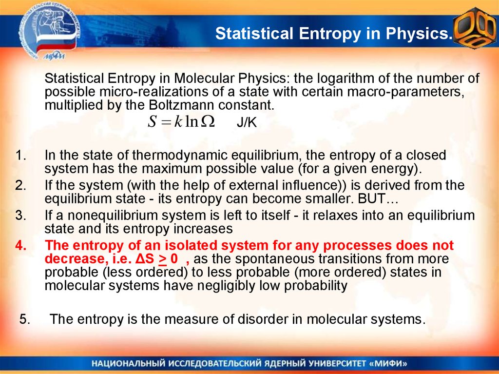
Statistical Entropy in Physics.
Statistical Entropy in Molecular Physics: the logarithm of the number of
possible micro-realizations of a state with certain macro-parameters,
multiplied by the Boltzmann constant.
S k ln J/K
1.
2.
3.
4.
5.
In the state of thermodynamic equilibrium, the entropy of a closed
system has the maximum possible value (for a given energy).
If the system (with the help of external influence)) is derived from the
equilibrium state - its entropy can become smaller. BUT…
If a nonequilibrium system is left to itself - it relaxes into an equilibrium
state and its entropy increases
The entropy of an isolated system for any processes does not
decrease, i.e. ΔS > 0 , as the spontaneous transitions from more
probable (less ordered) to less probable (more ordered) states in
molecular systems have negligibly low probability
The entropy is the measure of disorder in molecular systems.

6.

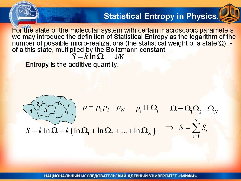
Statistical Entropy in Physics.
For the state of the molecular system with certain macroscopic parameters
we may introduce the definition of Statistical Entropy as the logarithm of the
number of possible micro-realizations (the statistical weight of a state Ώ) of a this state, multiplied by the Boltzmann constant.
S k ln J/К
Entropy is the additive quantity.
2
1
i
3
p p1 p2 ... pN
pi
i
1 2 ... N
N
S k ln k ln 1 ln 2 ... ln N
S Si
i 1

7.

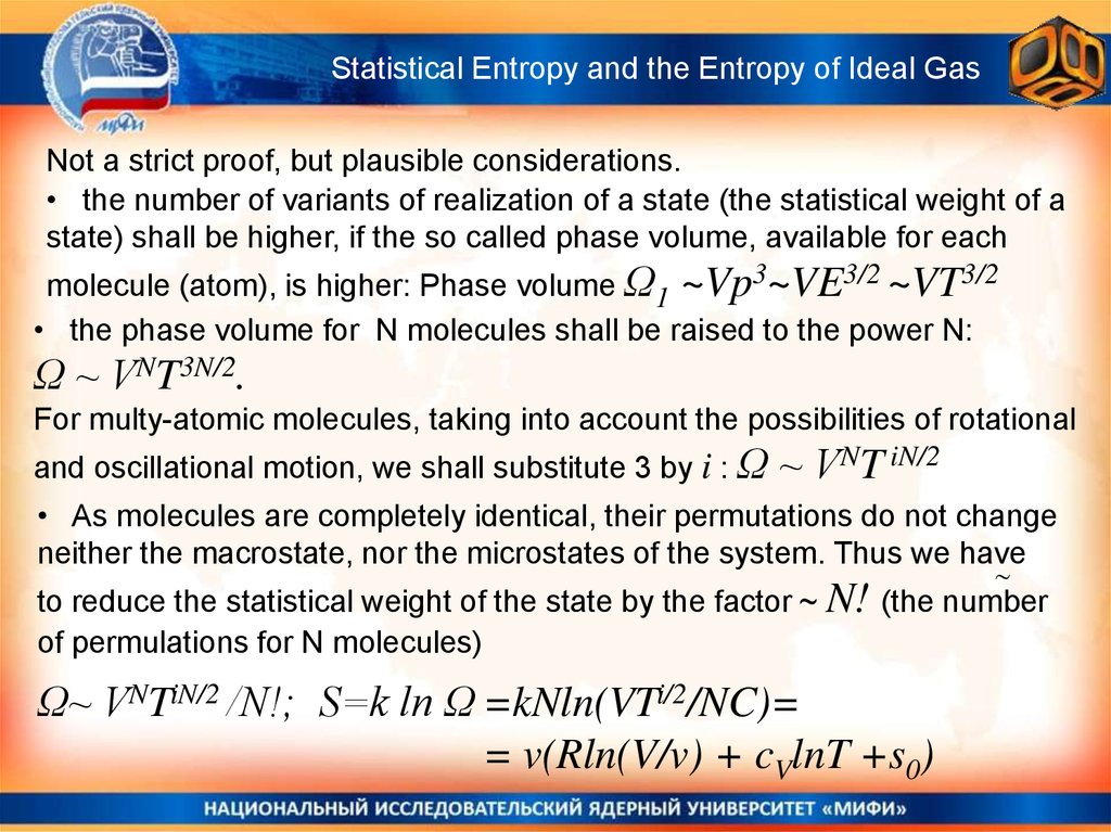
Statistical Entropy and the Entropy of Ideal Gas
Not a strict proof, but plausible considerations.
• the number of variants of realization of a state (the statistical weight of a
state) shall be higher, if the so called phase volume, available for each
molecule (atom), is higher: Phase volume Ω1 ~Vp3~VE3/2 ~VT3/2
• the phase volume for N molecules shall be raised to the power N:
Ω ~ VNT3N/2.
For multy-atomic molecules, taking into account the possibilities of rotational
and oscillational motion, we shall substitute 3 by i : Ω
~ VNT iN/2
• As molecules are completely identical, their permutations do not change
neither the macrostate, nor the microstates of the system. Thus we have
to reduce the statistical weight of the state by the factor ~ N! (the number
of permulations for N molecules)
Ω~ VNTiN/2 /N!; S=k ln Ω =kNln(VTi/2/NC)=
= v(Rln(V/v) + cVlnT +s0)

8.

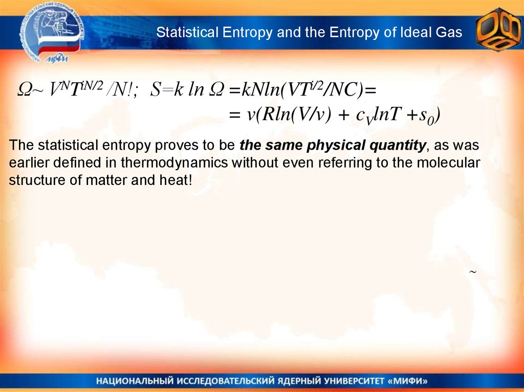
Statistical Entropy and the Entropy of Ideal Gas
Ω~ VNTiN/2 /N!; S=k ln Ω =kNln(VTi/2/NC)=
= v(Rln(V/v) + cVlnT +s0)
The statistical entropy proves to be the same physical quantity, as was
earlier defined in thermodynamics without even referring to the molecular
structure of matter and heat!

9.

MEPhI General Physics
The Distributions of Molecules
over Velocities and Energies
Maxwell and Boltzmann Distributions
That will be the Focus of the next lecture!

10.

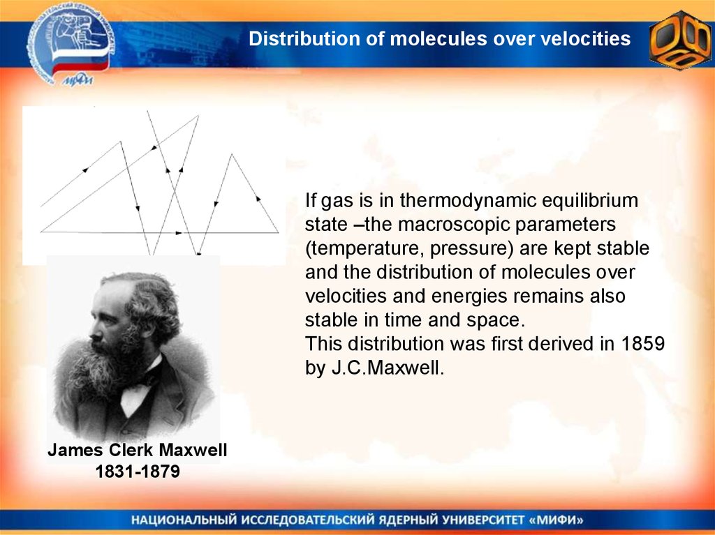
Distribution of molecules over velocities
If gas is in thermodynamic equilibrium
state –the macroscopic parameters
(temperature, pressure) are kept stable
and the distribution of molecules over
velocities and energies remains also
stable in time and space.
This distribution was first derived in 1859
by J.C.Maxwell.
James Clerk Maxwell
1831-1879

11.

Distribution of molecules over velocities
Each velocity vector can be presented as a point
in the velocity space,
As all the directions are equal – the distribution
function can not depend on the direction, but
only on the modulus of velocity
f(V)

12.

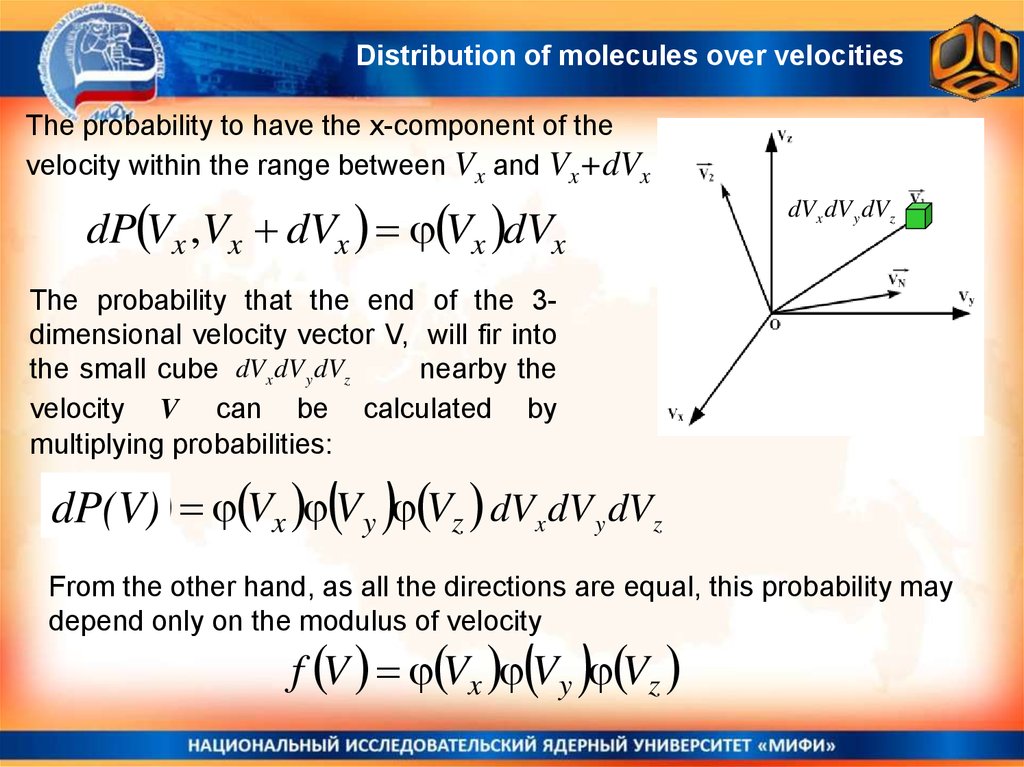
Distribution of molecules over velocities
The probability to have the x-component of the
velocity within the range between Vx and Vx+dVx
dP Vx ,Vx dVx Vx dVx
dVx dV y dVz
The probability that the end of the 3dimensional velocity vector V, will fir into
the small cube dVx dV y dVz
nearby the
velocity V can be calculated by
multiplying probabilities:
f V Vx Vy Vz dVx dV y dVz
dP(V)
From the other hand, as all the directions are equal, this probability may
depend only on the modulus of velocity
f V Vx Vy Vz

13.

Distribution of molecules over velocities
Noe some mathematics:
f V Vx Vy Vz
dVx dV y dVz
ln( f (V )) ln( (Vx )) ln( (Vy )) ln( (Vz ))
We will calculate the derivative by dVx
Vx
f V V
f V Vx Vx
as
f V 1 Vx 1
f V V Vx Vx
Vx
Vx
V
2
2
2
Vx
V
Vx V y Vz

14.

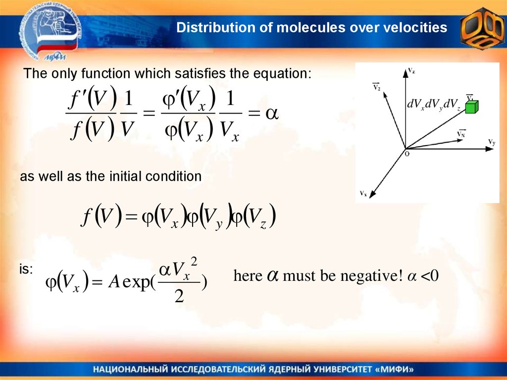
Distribution of molecules over velocities
The only function which satisfies the equation:
f V 1 Vx 1
f V V Vx Vx
dVx dV y dVz
as well as the initial condition
f V Vx Vy Vz
is:
V x 2
Vx A exp(
)
2
here α must be negative! α <0

15.

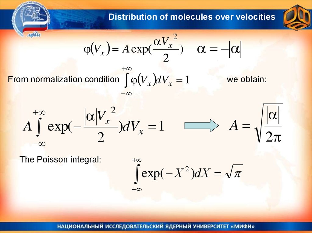
Distribution of molecules over velocities
V x
Vx A exp(
)
2
2
From normalization condition
: Vx dVx 1
we obtain:
Vx
A exp(
)dVx 1
2
The Poisson integral:
2
A
2
2
exp(
Х
)dХ

16.

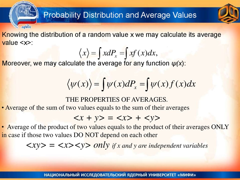
Probability Distribution and Average Values
Knowing the distribution of a random value x we may calculate its average
value <x>:
x xdPx xf ( x)dx,
Moreover, we may calculate the average for any function ψ(x):
( x) ( x)dPx ( x) f ( x)dx
THE PROPERTIES OF AVERAGES.
• Average of the sum of two values equals to the sum of their averages
<x + y> = <x> + <y>
• Average of the product of two values equals to the product of their averages ONLY
in case if those two values DO NOT depend on each other
<xy> = <x><y> only if x and y are independent variables

17.

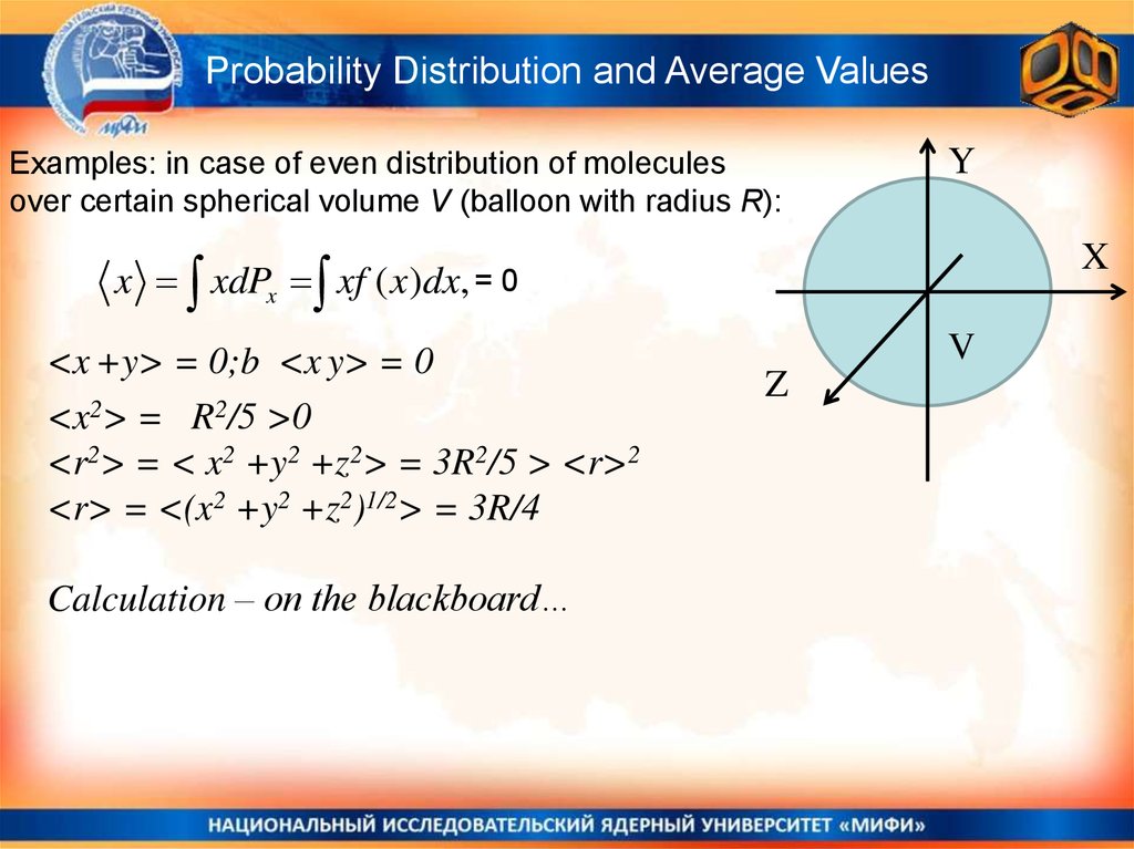
Probability Distribution and Average Values
Examples: in case of even distribution of molecules
over certain spherical volume V (balloon with radius R):
Y
X
x xdPx xf ( x)dx, = 0
<x +y> = 0;b <x y> = 0
<x2> = R2/5 >0
<r2> = < x2 +y2 +z2> = 3R2/5 > <r>2
<r> = <(x2 +y2 +z2)1/2> = 3R/4
Calculation – on the blackboard…
V
Z

18.

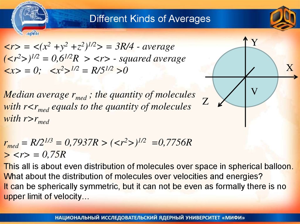
Different Kinds of Averages
<r> = <(x2 +y2 +z2)1/2> = 3R/4 - average
(<r2>)1/2 = 0,61/2R > <r> - squared average
<x> = 0; <x2>1/2 = R/51/2 >0
Y
Median average rmed ; the quantity of molecules
with r<rmed equals to the quantity of molecules Z
with r>rmed
V
X
rmed = R/21/3 = 0,7937R > (<r2>)1/2 =0,7756R
> <r> = 0,75R
This all is about even distribution of molecules over space in spherical balloon.
What about the distribution of molecules over velocities and energies?
It can be spherically symmetric, but it can not be even as formally there is no
upper limit of velocity…

19.

Distribution of molecules over velocities
V x
Vx A exp(
)
2
2
A
2
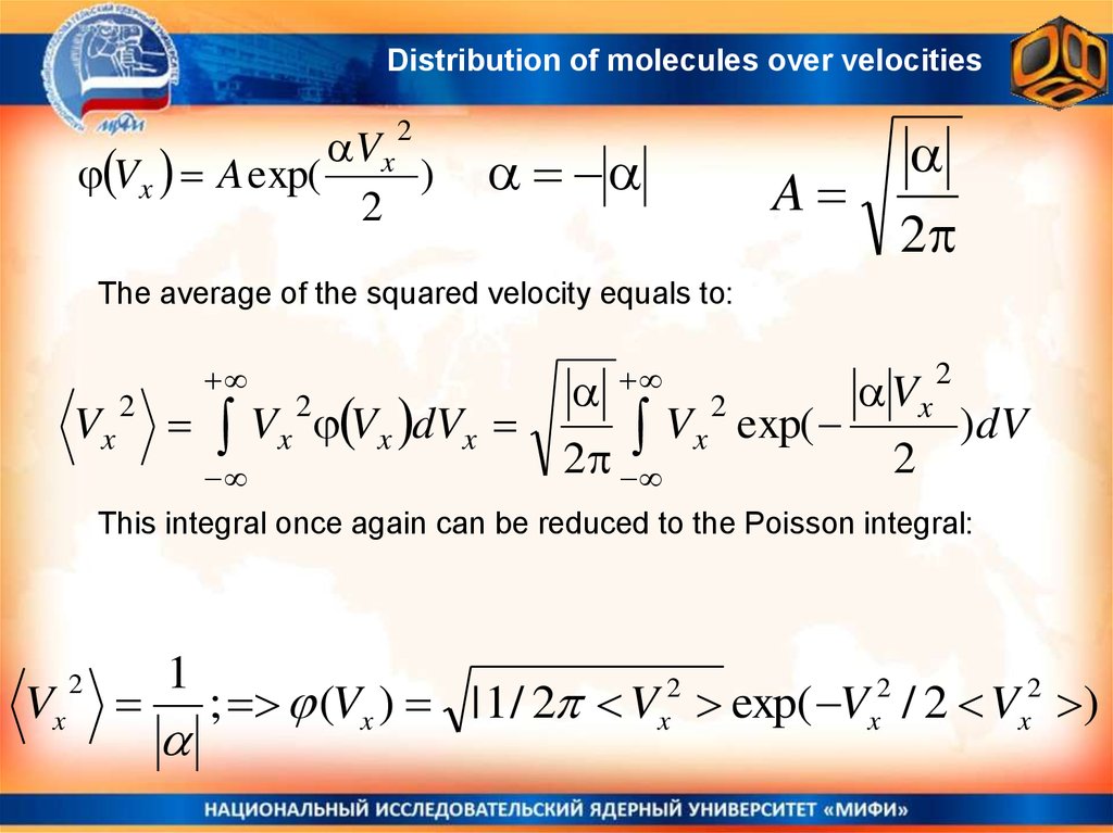
The average of the squared velocity equals to:
Vx 2
Vx 2 Vx dVx
2
Vx 2
Vx exp(
)dV
2
2
This integral once again can be reduced to the Poisson integral:
Vx
2
1
; (Vx ) | 1 / 2 V exp( V / 2 V )
2
x
2
x
2
x

20.

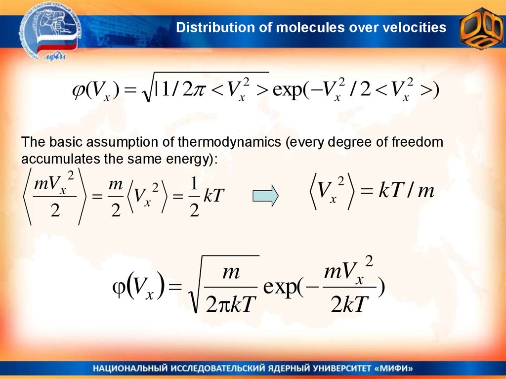
Distribution of molecules over velocities
(Vx ) | 1 / 2 V exp( V / 2 V )
2
x
2
x
2
x
The basic assumption of thermodynamics (every degree of freedom
accumulates the same energy):
mV x
2
2
m
1
2
Vx kT
2
2
Vx
2
kT / m
2
mVx
m
Vx
exp(
)
2 kT
2kT

21.

Distribution of molecules over velocities
2
mVx
m
Vx
exp(
)
2 kT
2kT
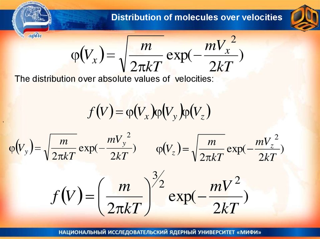
The distribution over absolute values of velocities:
f V Vx Vy Vz
,
mV y 2
m
Vy
exp(
)
2 kT
2kT
m
f V
2 kT
m
mVz 2
Vz
exp(
)
2 kT
2kT
3
2
2
mV
exp(
)
2kT

22.

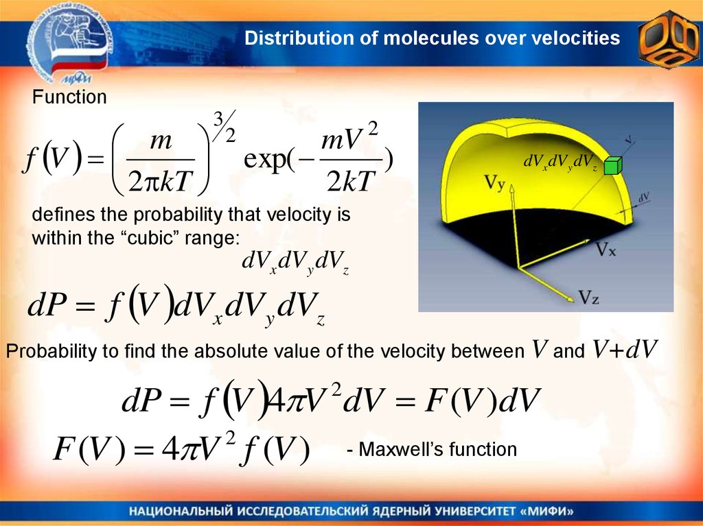
Distribution of molecules over velocities
Function
m
f V
2 kT
3
2
2
mV
exp(
)
2kT
dVx dV y dVz
defines the probability that velocity is
within the “cubic” range:
dVx dV y dVz
dP f V dVx dVy dVz
Probability to find the absolute value of the velocity between V and V+dV
dP f V 4 V dV F (V )dV
2
F (V ) 4 V f (V ) - Maxwell’s function
2

23.

Maxwell’s Function
m
F V
2 kT
3
2
mV 2
4 V 2
exp
2
kT
V Vвер
F V V
2
V Vвер
mV 2
F V exp
2
kT

24.

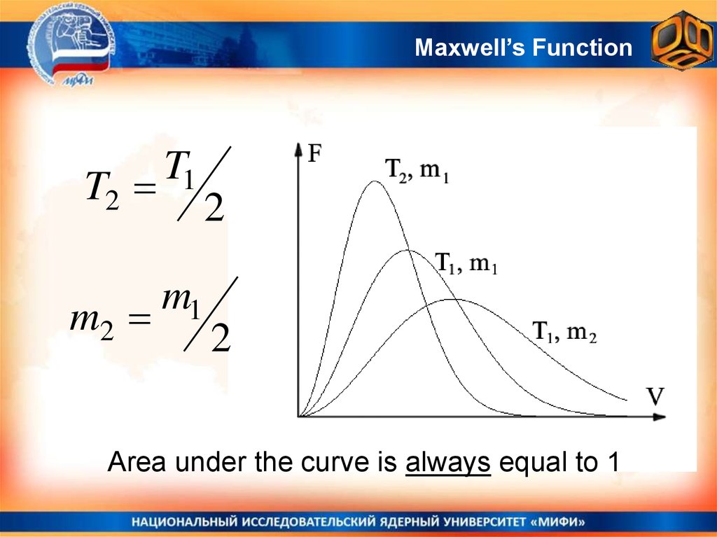
Maxwell’s Function
T
T2 1
2
m
m2 1
2
Area under the curve is always equal to 1

25. Stern’s experiment (1920)

• The outer cylinder is rotating
S R t
R
t
V
R 2
V
S

26. Lammert’s Experiment (1929)

• Two rotating discs with radial slots. One is rotating
ahead of the other. The angle distance is
t1 l
V
t2 l
V l

27. Most probable velocity.

Most probable velocity corresponds to the maximum of the Maxwell’s
function)
dF v
mV 2
mV 2
m 2
4
2
0
V exp
dv
kT
2 kT
2kT
3
Most probable velocity
Vвер
2kT
m
The value of the Maxwell’s function maximum:
F vвер
4
m
4 1
e 2kT
e vвер
Vвер

28. Average velocity.

Average velocity by deffinition
V VdP VF V dV
For Maxwell’s function:
0
3
2
2
mV
m
3
V 4
dV
V exp
2 kT 0
2kT
8kT
V
m

29.

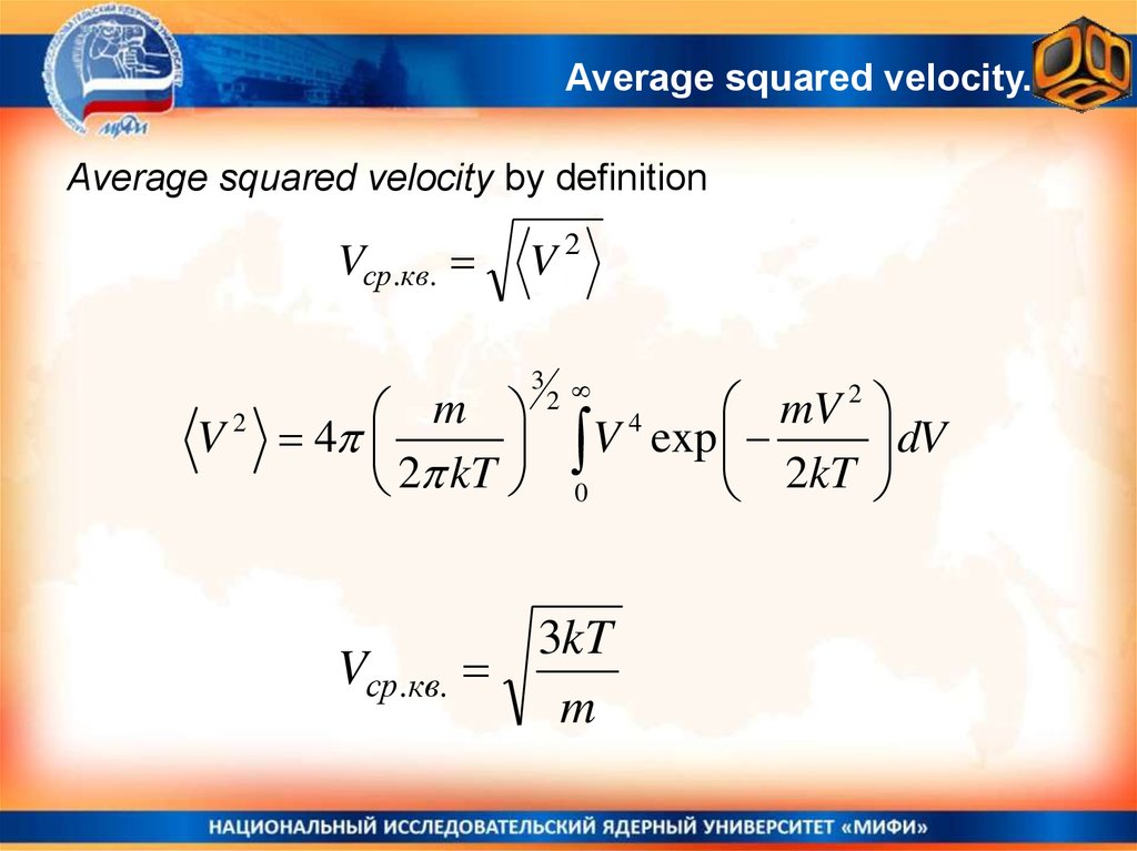
Average squared velocity.
Average squared velocity by definition
Vср.кв.
V2
3
V2
2
2
mV
m
4
4
dV
V exp
2 kT 0
2kT
Vср.кв.
3kT
m

30.

Three kinds of average velocities
2kT
m
Most probable:
Vвер
Averge:
8kT
V
m
Average squared:
Vср.кв.
3kT
m

31.

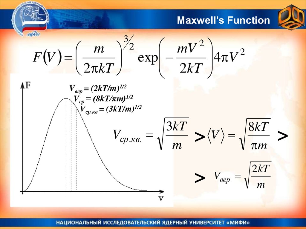
Maxwell’s Function
m
F V
2 kT
3
2
mV 2
2
exp
4
V
2
kT
Vвер = (2kT/m)1/2
Vср = (8kT/πm)1/2
Vср.кв = (3kT/m)1/2
Vср.кв.
3kT
m
>
8kT
V
m
>
2kT
m
Vвер
>

32.

Example:
Example: The mixture of oxygen and nitrogen (air) has the
temperature T = 300 K. What are the average velocities of two types
of molecules:
VO
2
8kT
mO
2
VO
VN
2
2
VN
2
8kT
mN
8 8,31 300
3 м
м
0
,
45
10
450
с
с
3,14 32 10 3
8 8,31 300
3 м
0
,
48
10
480 м
3
с
с
3,14 28 10
2

33.

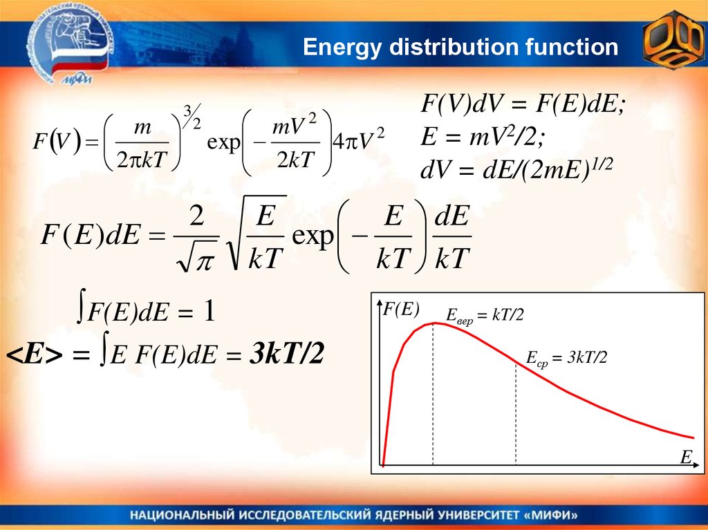
Energy distribution function
m
F V
2 kT
F ( E )dE
3
2
mV
exp
2kT
2
2
4 V 2
F(V)dV = F(E)dE;
E = mV2/2;
dV = dE/(2mE)1/2
E
E dE
exp
kT
kT kT
∫F(E)dE = 1
<E> = ∫E F(E)dE = 3kT/2
F(E)
Eвер = kT/2
Eср = 3kT/2
E

34.

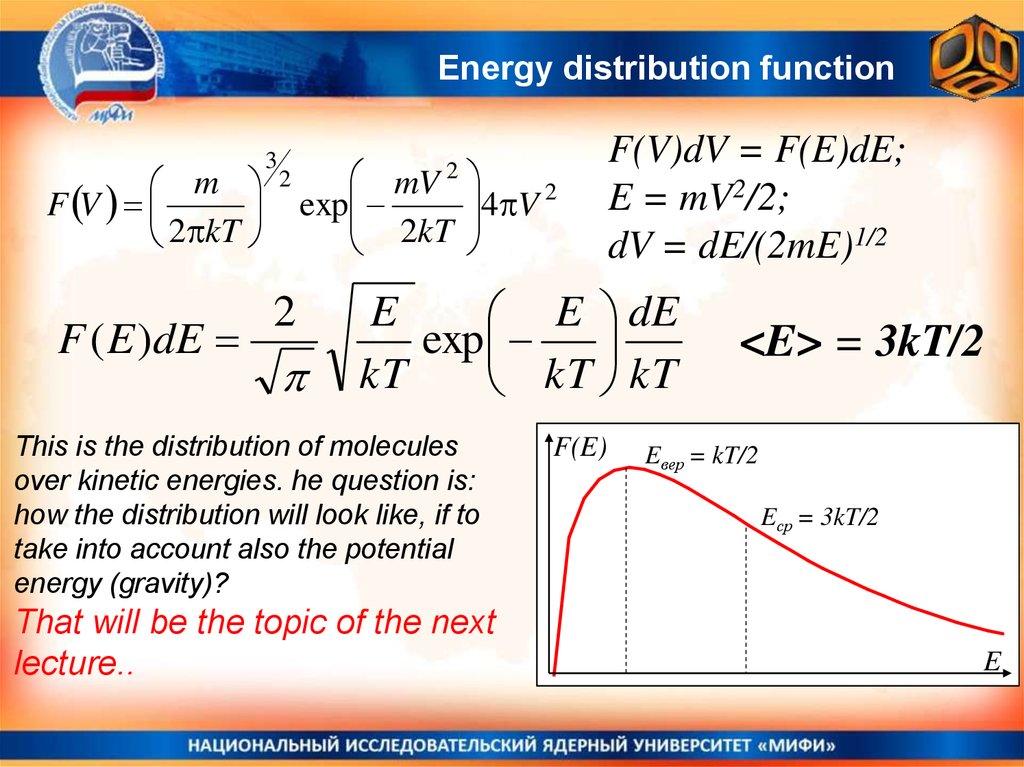
Energy distribution function
m
F V
2 kT
F ( E )dE
3
2
mV
exp
2kT
2
2
4 V 2
F(V)dV = F(E)dE;
E = mV2/2;
dV = dE/(2mE)1/2
E
E dE
exp
kT
kT kT
This is the distribution of molecules
over kinetic energies. he question is:
how the distribution will look like, if to
take into account also the potential
energy (gravity)?
That will be the topic of the next
lecture..
F(E)
<E> = 3kT/2
Eвер = kT/2
Eср = 3kT/2
E

35.

Thank You for Attention!