D2D wireless connection modeling for moving devices in 5G technology

1. D2D wireless connection modeling for moving devices in 5G technology

Sergey L. Fedorov
Keldysh Institute of Applied Mathematics of RAS
D2D wireless connection modeling
for moving devices in 5G technology
1. Non-stationary random walk trajectories modeling
2. SIR Indicator trajectory
3. Distribution of SIR Indicator
4. Distribution of the first break down moment
5. Cashing effects

2. The problem in general

2

3.

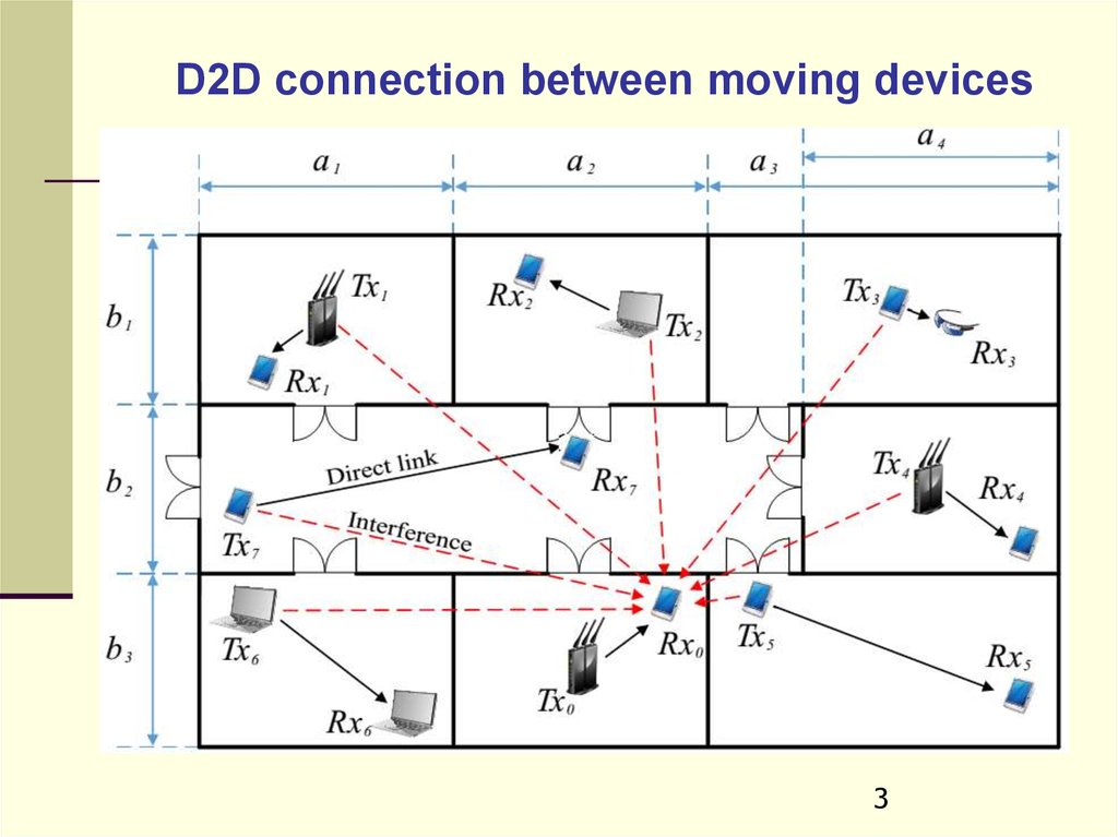
D2D connection between moving devices
3

4.

The main steps of modeling
1. Construction of the Fokker-Planck equation, based on the empirical
data about subscribers motion.
2. Estimation of the so-called self-consistent stationary level (SCSL) of
subscribers random walk.
3. Numerical solution of Fokker-Planck equation over the horizon with
the accuracy, which does not exceed SCSL.
4. Construction of the time series trajectory with the use of timedepending distribution function as a solution of kinetic equation.
5. Calculation of the functional, depending on the ensemble of
trajectories.
6. Solution of various problems of stochastic control.
•4

5. Generation of non-stationary trajectories of random walk

5

6.

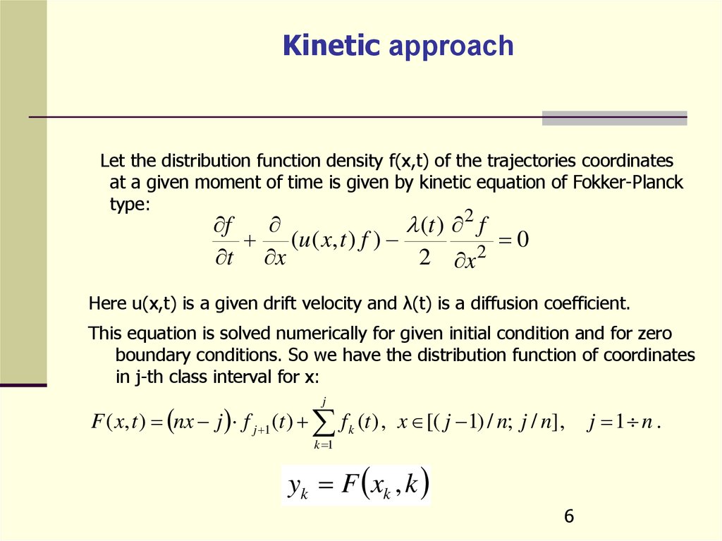
Kinetic approach
Let the distribution function density f(x,t) of the trajectories coordinates
at a given moment of time is given by kinetic equation of Fokker-Planck
type:
2
f
(t ) f
(u ( x, t ) f )
0
2
t x
2 x
Here u(x,t) is a given drift velocity and λ(t) is a diffusion coefficient.
This equation is solved numerically for given initial condition and for zero
boundary conditions. So we have the distribution function of coordinates
in j-th class interval for x:
j
F ( x, t ) nx j f j 1 (t ) f k (t ) , x [( j 1) / n; j / n] ,
k 1
yk F xk , k
6
j 1 n .

7.

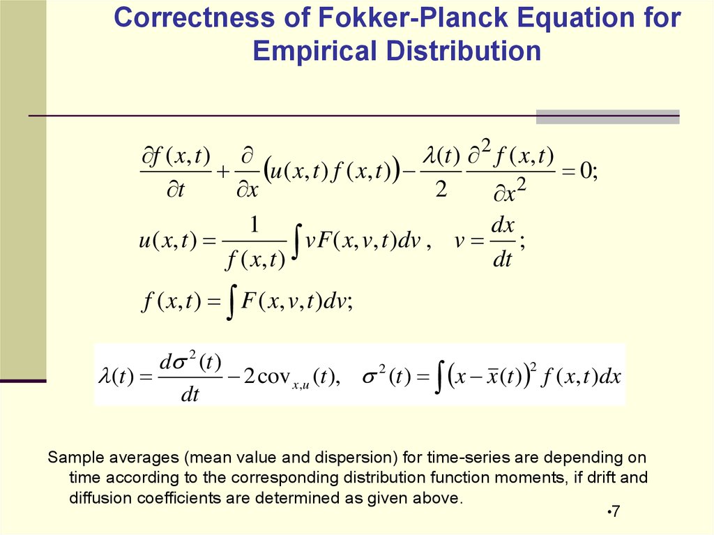
Correctness of Fokker-Planck Equation for
Empirical Distribution
f ( x, t )
(t ) 2 f ( x, t )
u ( x, t ) f ( x, t )
0;
t
x
2
x 2
1
dx
u ( x, t )
vF ( x, v, t )dv , v ;
f ( x, t )
dt
f ( x, t ) F ( x, v, t )dv;
d 2 (t )
2
(t )
2 cov x ,u (t ), 2 (t ) x x (t ) f ( x, t )dx
dt
Sample averages (mean value and dispersion) for time-series are depending on
time according to the corresponding distribution function moments, if drift and
diffusion coefficients are determined as given above.
•7

8.

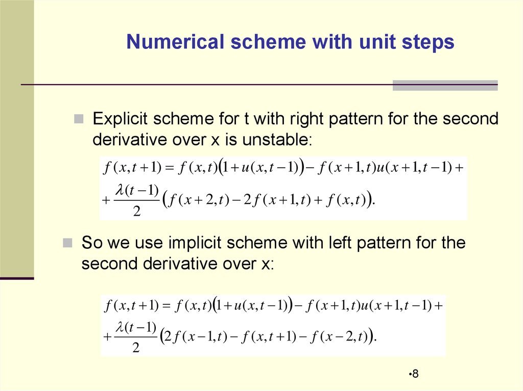
Numerical scheme with unit steps
Explicit scheme for t with right pattern for the second
derivative over x is unstable:
f ( x, t 1) f ( x, t ) 1 u ( x, t 1) f ( x 1, t )u ( x 1, t 1)
(t 1)
2
f ( x 2, t ) 2 f ( x 1, t ) f ( x, t ) .
So we use implicit scheme with left pattern for the
second derivative over x:
f ( x, t 1) f ( x, t ) 1 u ( x, t 1) f ( x 1, t )u ( x 1, t 1)
(t 1)
2
2 f ( x 1, t ) f ( x, t 1) f ( x 2, t ) .
•8

9.

Typical example of drift u(x,t)
0,01
0,006
0,004
0,002
0,32
0,30
0,28
0,26
0,24
0,22
0,20
0,18
0,16
0,14
0,12
0,10
0,08
0,06
0,04
-0,002
0,02
0
0,00
rate of variation of DF
0,008
-0,004
-0,006
normalized value of coordinate difference
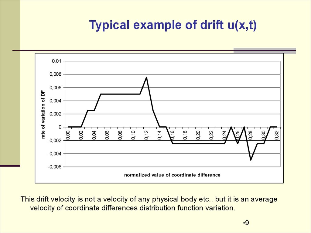
This drift velocity is not a velocity of any physical body etc., but it is an average
velocity of coordinate differences distribution function variation.
•9

10.

Probability Density Evolution Model
0,25
Probability
0,20
0,15
f1
f2
0,10
0,05
0,00
0,0
0,1
0,2
0,3
0,4
0,5
0,6
0,7
0,8
0,9
1,0
Coordinate difference
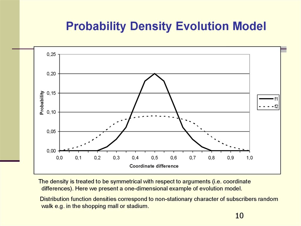
The density is treated to be symmetrical with respect to arguments (i.e. coordinate
differences). Here we present a one-dimensional example of evolution model.
Distribution function densities correspond to non-stationary character of subscribers random
walk e.g. in the shopping mall or stadium.
10

11.

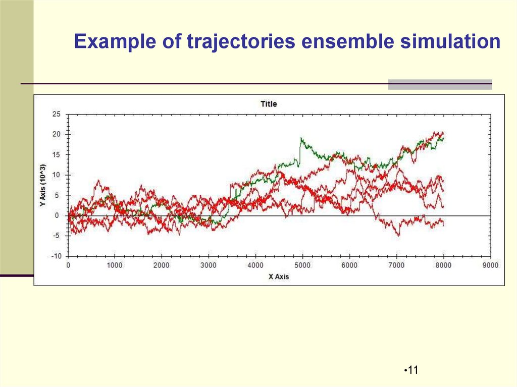
Example of trajectories ensemble simulation
•11

12. SCSL definition in C norm

N (t ) FN ( x, t N ) FN ( x, t )
For any given set volume N we construct the distribution function
G of distances between distribution functions F at various moments
of time
GN ( )
and we define SCSL
*(N )
from the following equation:
GN 1
*
*
•12

13.

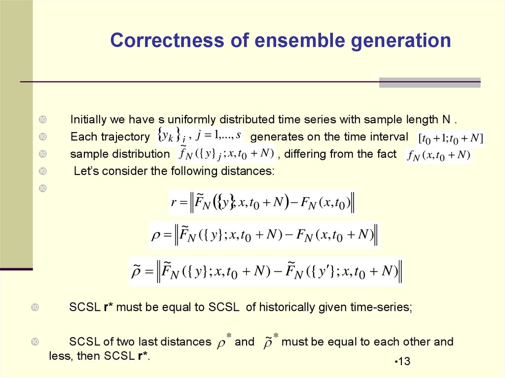
Correctness of ensemble generation
Initially we have s uniformly distributed time series with sample length N .
Each trajectory y k j , j 1,..., s generates on the time interval [t0 1; t0 N ]
~
sample distribution f N ({ y} j ; x, t 0 N ) , differing from the fact f N ( x, t 0 N )
Let’s consider the following distances:
~
r FN y ; x, t0 N FN ( x, t0 )
~
FN ({ y}; x, t 0 N ) FN ( x, t 0 N )
~
~
~
FN ({ y}; x, t 0 N ) FN ({ y }; x, t 0 N )
SCSL r* must be equal to SCSL of historically given time-series;
SCSL of two last distances
less, then SCSL r*.
* and ~ * must be equal to each other and
•13

14. SIR Indicator Trajectory

14

15.

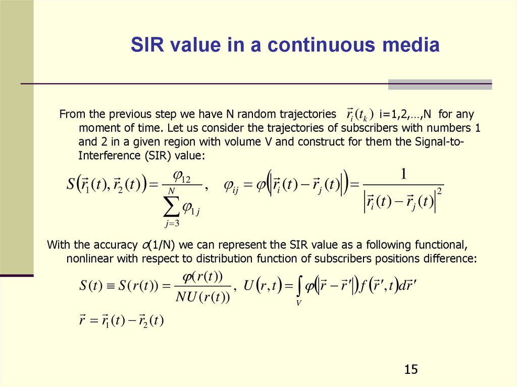
SIR value in a continuous media
From the previous step we have N random trajectories ri (t k ) i=1,2,…,N for any
moment of time. Let us consider the trajectories of subscribers with numbers 1
and 2 in a given region with volume V and construct for them the Signal-toInterference (SIR) value:
1
S r1 (t ), r2 (t ) N 12 , ij ri (t ) rj (t )
2
ri (t ) rj (t )
j 3
1j
With the accuracy o(1/N) we can represent the SIR value as a following functional,
nonlinear with respect to distribution function of subscribers positions difference:
S (t ) S (r (t ))
r r1 (t ) r2 (t )
(r (t ))
NU (r (t ))
, U r , t r r f r , t dr
V
15

16.

Example of 10 trajectories in square with
reflection boundary conditions
•16

17.

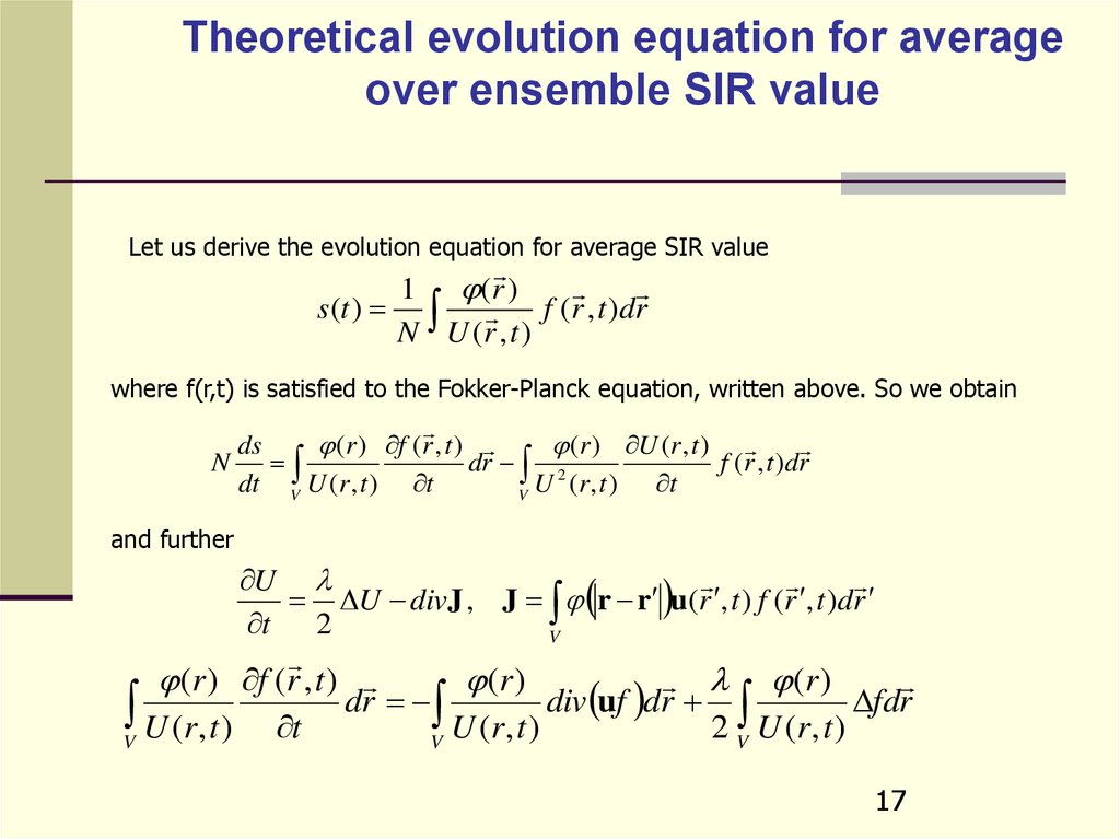
Theoretical evolution equation for average
over ensemble SIR value
Let us derive the evolution equation for average SIR value
1 (r )
s(t ) f (r , t )dr
N U (r , t )
where f(r,t) is satisfied to the Fokker-Planck equation, written above. So we obtain
ds
(r ) f (r , t )
(r ) U (r , t )
N
dr 2
f (r , t )dr
dt V U (r , t ) t
U (r , t ) t
V
and further
U
U divJ , J r r u(r , t ) f (r , t )dr
t
2
V
(r ) f (r , t )
U (r , t )
V
t
(r )
(r )
dr
div uf dr
fdr
U (r , t )
2 V U (r , t )
V
17

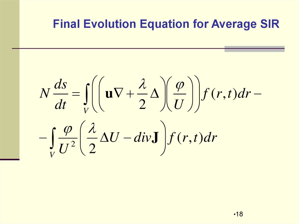
18.

Final Evolution Equation for Average SIR
ds
N
u
dt V
2 U
f (r , t )dr
2 U divJ f (r , t )dr
U 2
V
•18

19.

SIR dispersion evolution equation – 1
Let us consider a SIR variance
2
1 (x)
(x )
2
(t )
f (x , t )dx f (x, t )dx
N 2 V U (x, t ) V U (x , t )
Then we obtain
N2
2
f (x, t )
d (t ) (x)
Ns(t )
dx
dt
U (x, t )
t
V
2
(x) U (x, t )
ds(t ) (x)
2 2
N
Ns(t ) f (x, t )dx .
U (x, t ) t
dt U (x, t )
V
And finally
19

20.

SIR dispersion evolution equation – 2
d 2 (t )
( x)
( x)
( x)
u(x, t )
N
2
2
div x J f (x, t )dx
dt
U (x, t )
U (x, t ) U (x, t )
V
2
( x)
( x)
f (x, t )dx
2 Ns(t ) 2
div x J u(x, t )
U (x, t )
U ( x, t )
V
( x)
( x)
f (x, t )dx
Ns(t ) (t ) 2
U
U (x, t )
U (x, t )
V
2
2
( x)
(
x
)
(
x
)
( x)
3
(t )
U f (x, t )dx .
U (x, t ) U (x, t ) U (x, t ) U (x, t )
V
So we see, that it is very complex non-linear with respect to f(x,t) equation and its
theoretical investigation is very difficult. Hence we need to numerical simulation of
various regimes of D2D connection.
20

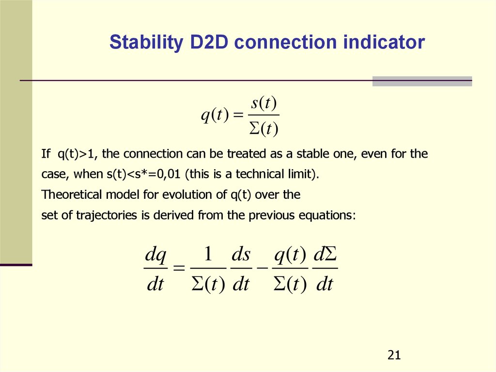
21.

Stability D2D connection indicator
s (t )
q(t )
(t )
If q(t)>1, the connection can be treated as a stable one, even for the
case, when s(t)<s*=0,01 (this is a technical limit).
Theoretical model for evolution of q(t) over the
set of trajectories is derived from the previous equations:
dq
1 ds q(t ) d
dt (t ) dt (t ) dt
21

22. SIR Indicator Distribution Function

22

23.

Typical SIR trajectory and SIR distribution
•23

24.

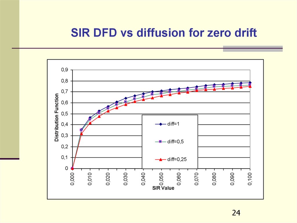
SIR DFD vs diffusion for zero drift
0,9
0,7
0,6
0,5
diff=1
0,4
0,3
diff=0,5
0,2
0,1
diff=0,25
SIR Value
24
0,100
0,090
0,080
0,070
0,060
0,050
0,040
0,030
0,020
0,010
0
0,000
Distribution Function
0,8

25.

0,045
0,040
0,035
0,030
0,025
0,020
0,015
0,010
0,005
0,000
SIR Value
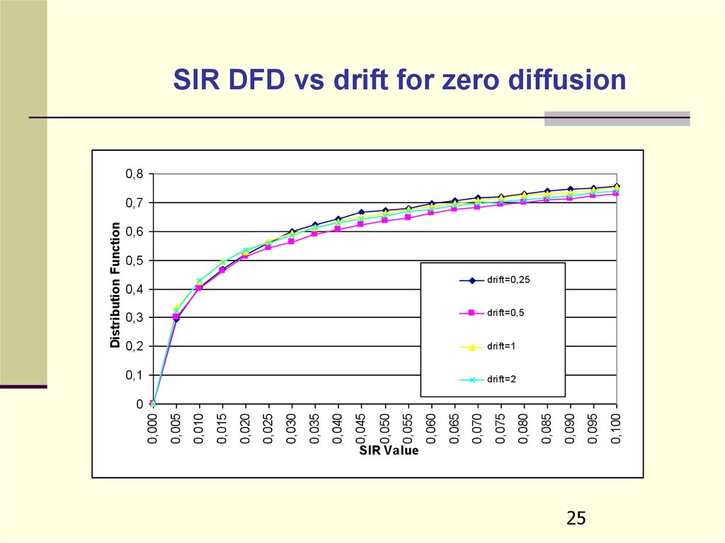
drift=1
0,1
drift=2
25
0,100
0,2
0,095
drift=0,5
0,090
0,3
0,085
0,080
0,4
0,075
0,070
0,065
0,060
0,055
0,050
Distribution Function
SIR DFD vs drift for zero diffusion
0,8
0,7
0,6
0,5
drift=0,25
0

26. Analysis of D2D connection stability

26

27.

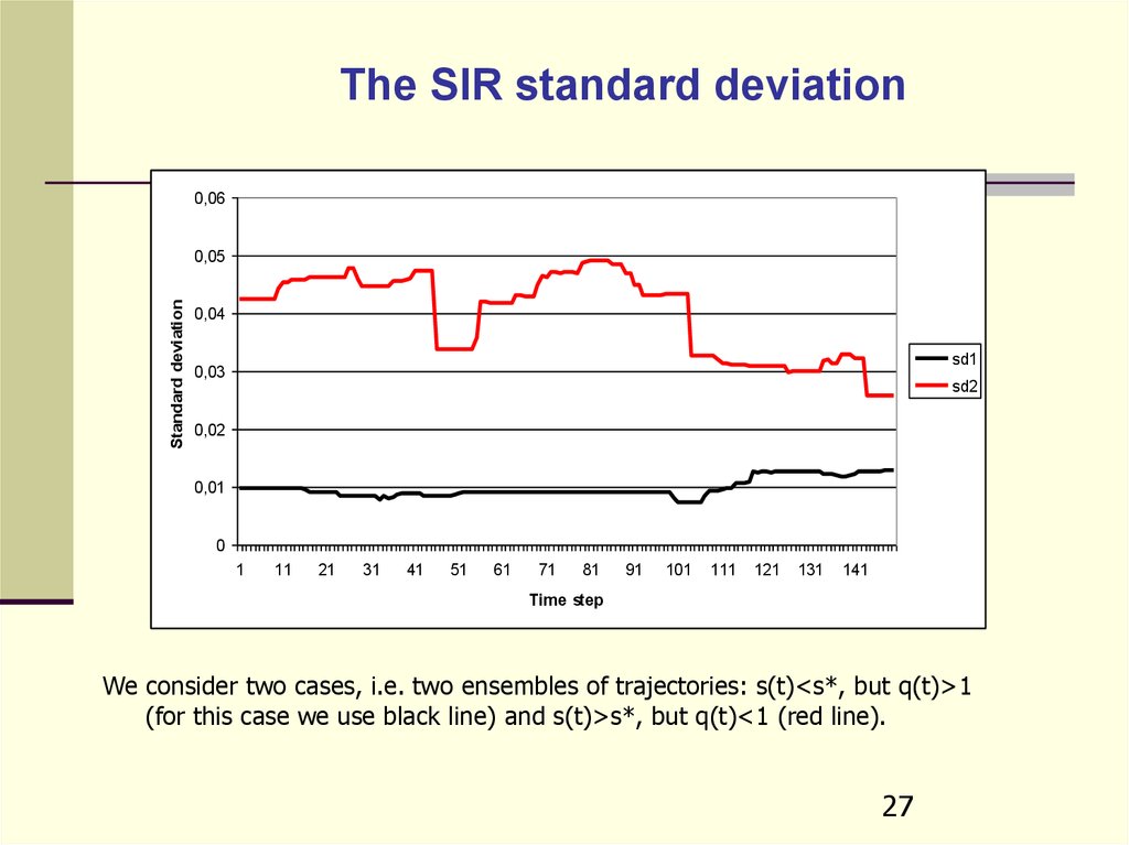
The SIR standard deviation
0,06
Standard deviation
0,05
0,04
sd1
0,03
sd2
0,02
0,01
0
1
11
21
31
41
51
61
71
81
91
101
111
121
131
141
Time step
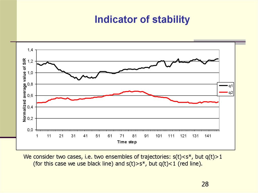
We consider two cases, i.e. two ensembles of trajectories: s(t)<s*, but q(t)>1
(for this case we use black line) and s(t)>s*, but q(t)<1 (red line).
27

28.

Indicator of stability
Normalized average value of SIR
1,4
1,2
1,0
0,8
q1
q2
0,6
0,4
0,2
0,0
1
11
21
31
41
51
61
71
81
Time step
91
101
111
121
131
141
We consider two cases, i.e. two ensembles of trajectories: s(t)<s*, but q(t)>1
(for this case we use black line) and s(t)>s*, but q(t)<1 (red line).
28

29.

The SIR Simulation
0,030
0,025
SIR value
0,020
avr1
0,015
sir1
0,010
S (t )
0,005
(r (t ))
NU (r (t ))
, N 10
0,000
1
11
21
31
41
51
61
71
81
91
101
111
121
131
141
Time step
0,06
0,05
SIR value
0,04
avr2
0,03
The first case (q>1) is more
stable, than the second one
(q<1): only 20% of the SIR
trajectory lies below the
critical line in the first case,
and 30% in the second.
sir2
0,02
0,01
0
1
11
21
31
41
51
61
71
81
91
101
111
121
131
141
Time step
29

30. Distribution Function of the first break down moment

30

31.

Simulation of empirical distribution function
of the first break down moment
S scr 0,01
1
0,9
Distribution Function
0,8
0,7
0,6
F1
0,5
F2
0,4
0,3
0,2
0,1
0
0
1
2
3
4
5
6
7
8
9
10
11
12
13
14
15
16
17
18
19
20
Time step
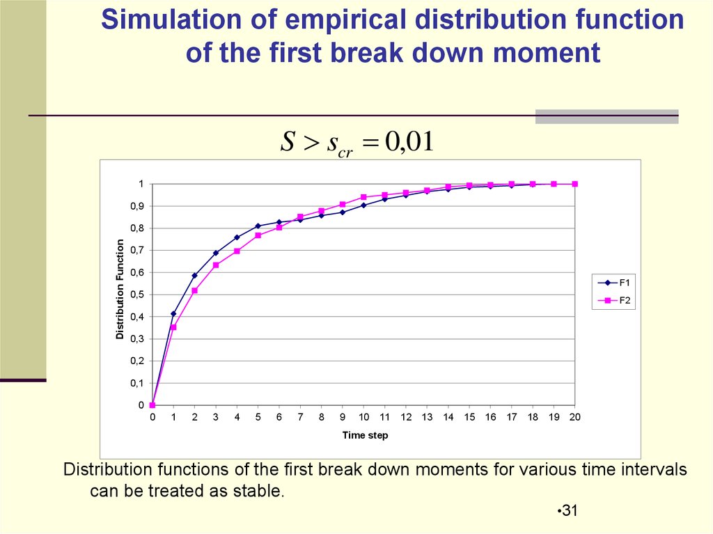
Distribution functions of the first break down moments for various time intervals
can be treated as stable.
•31

32.

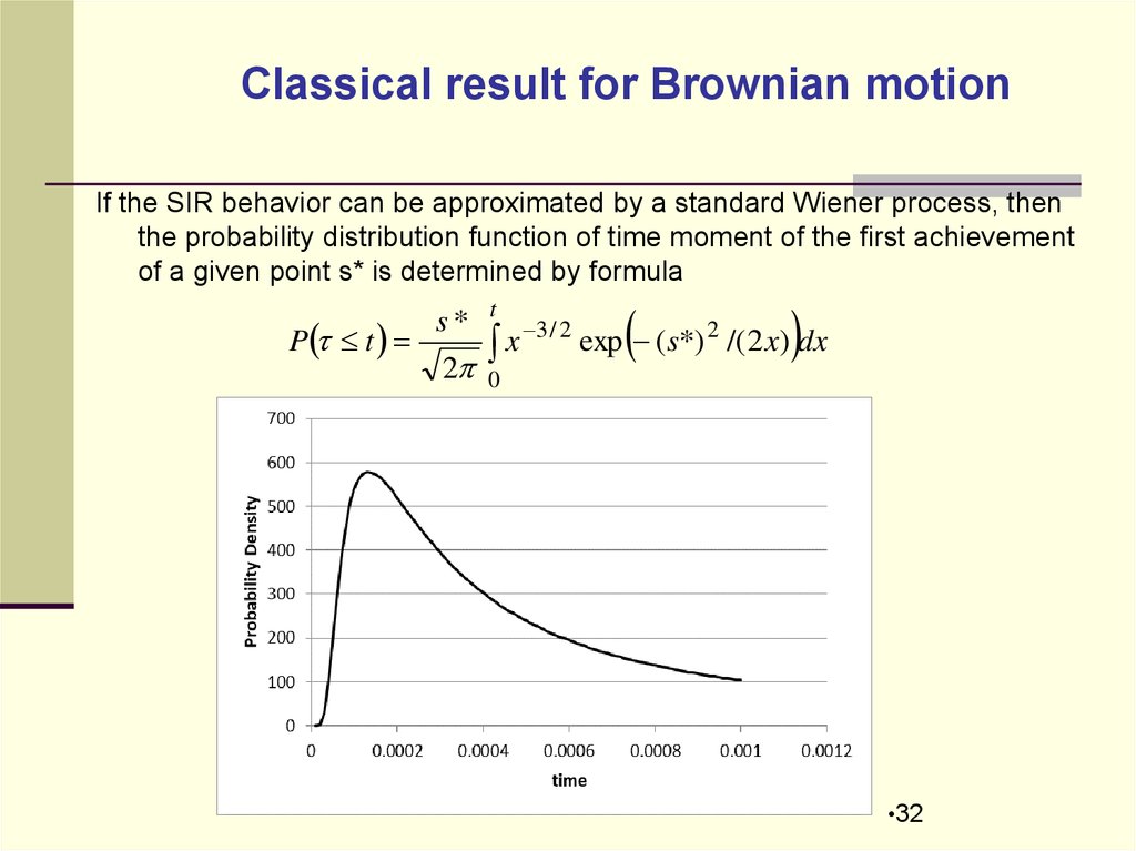
Classical result for Brownian motion
If the SIR behavior can be approximated by a standard Wiener process, then
the probability distribution function of time moment of the first achievement
of a given point s* is determined by formula
P t
s*
2
t
3 / 2
2
x
exp
(
s
*)
/( 2 x) dx
0
•32

33.

Simulation DFD for non-stationary random
walk of subscribers
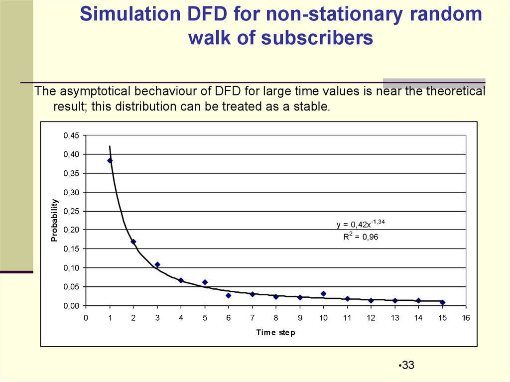
The asymptotical bechaviour of DFD for large time values is near the theoretical
result; this distribution can be treated as a stable.
0,45
0,40
0,35
Probability
0,30
0,25
y = 0,42x -1,34
R2 = 0,96
0,20
0,15
0,10
0,05
0,00
0
1
2
3
4
5
6
7
8
9
10
11
12
13
14
Time step
•33
15
16

34. Analysis of cashing effects

34

35. Simulation results for DFD first break down with cashing

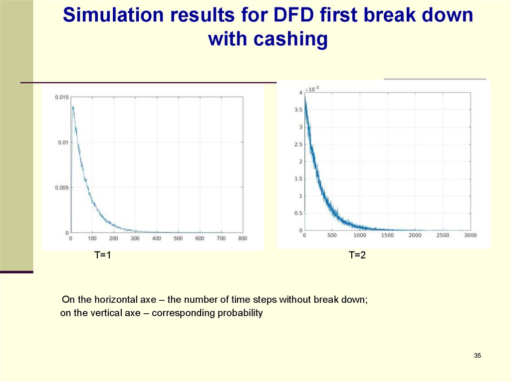
T=1
T=2
On the horizontal axe – the number of time steps without break down;
on the vertical axe – corresponding probability
35

36. Empirical dependence of the maximum continuity period on the cashing value

36

37. The type of normalized DFD

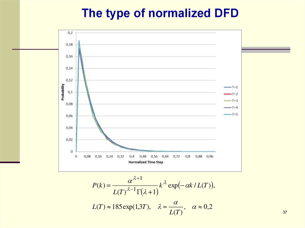
P(k )
1
L(T ) 1 1
k exp k / L(T ) ,
L(T ) 185 exp(1,3T ),
L(T )
, 0,2
37

38. Conclusions

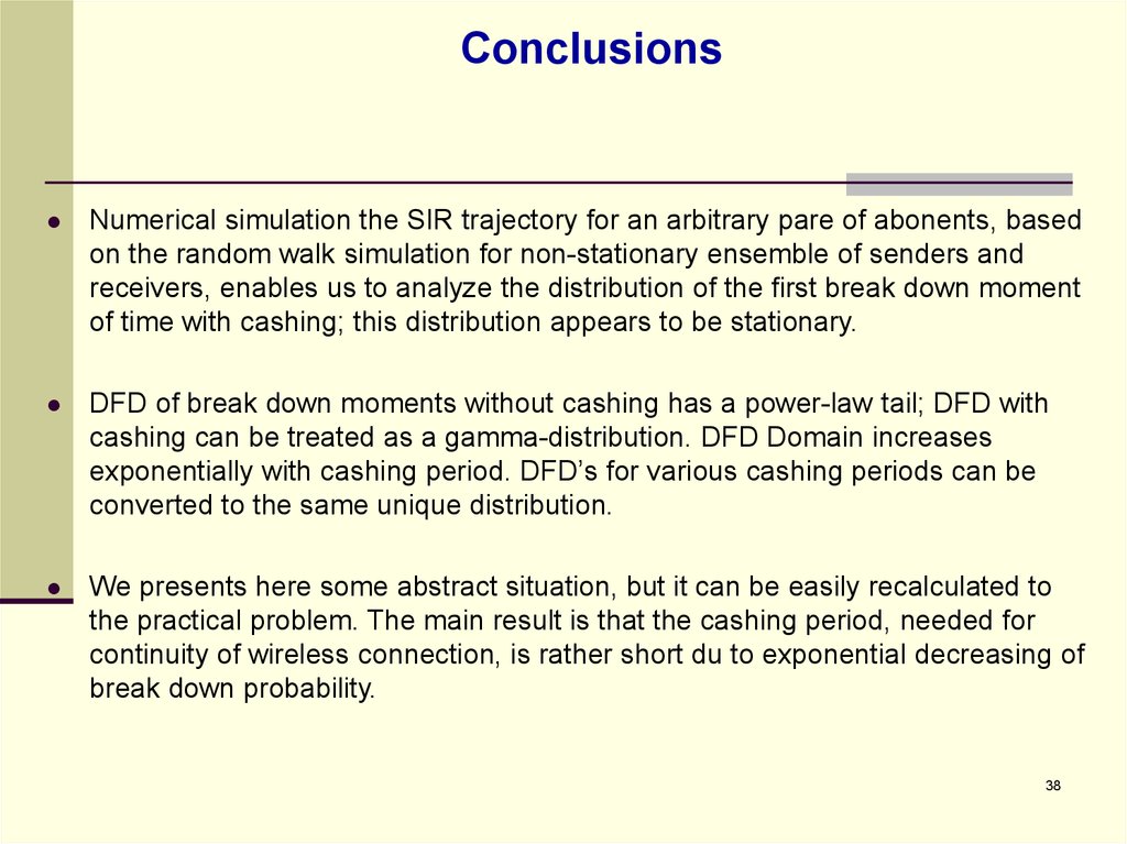
Numerical simulation the SIR trajectory for an arbitrary pare of abonents, based
on the random walk simulation for non-stationary ensemble of senders and
receivers, enables us to analyze the distribution of the first break down moment
of time with cashing; this distribution appears to be stationary.
DFD of break down moments without cashing has a power-law tail; DFD with
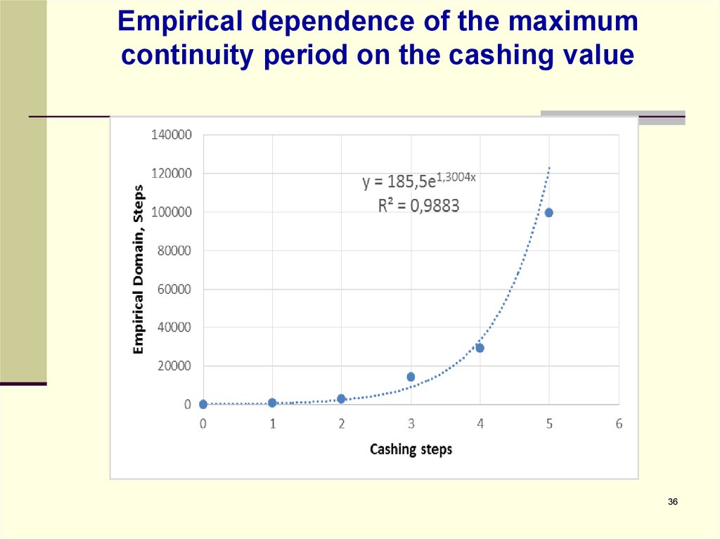
cashing can be treated as a gamma-distribution. DFD Domain increases
exponentially with cashing period. DFD’s for various cashing periods can be
converted to the same unique distribution.
We presents here some abstract situation, but it can be easily recalculated to
the practical problem. The main result is that the cashing period, needed for
continuity of wireless connection, is rather short du to exponential decreasing of
break down probability.
38

39.

The main references
1. Orlov Yu.N., Fedorov S.L. 2016. Modelirovanie raspredelenij funkcionalov na ansamble traektorij
nestatsionarnogo sluchainogo processa (in russian) // Preprints KIAM of RAS. № 101. 14 p.
URL: http://library.keldysh.ru/preprint.asp?id=2016-101
2. Yu. Gaidamaka, Yu. Orlov, S. Fedorov, A. Samuylov, D. Molchanov. 2016. Simulation of Devices
Mobility to Estimate Wireless Channel Quality Metrics in 5G Network. Proc. ICNAAM,
September 19-25, Rhodes, Greece.
3. Fedorov S.L., Orlov Yu.N. 2016. Metody chislennogo modelirovaniya processov nestatsionarnogo
sluchajnogo bluzhdaniya (in Russian). – Moscow: MIPT.
4. Orlov Yu.N., Fedorov S.L. 2016. Generation of non-stationary time-series trajectories on the
basis of Fokker-Planck equation (in Russian). Trudy MIPT, 8, No. 2, 126-133.
5. Orlov Yu.N., Fedorov S.L. 2016. Modelirovanie ansamblya nestacionarnyh traektorij s
pomoshch'yu uravneniya Fokkera-Planka (in Russian). Zhurnal Srednevolzhskogo
matematicheskogo obshchestva, No1.
6. Orlov Yu.N., Fedorov S.L. 2017. Modelirovanie ansamblia nestatsionarnyh sluchainyh traektorij s
ispolzovaniem uravnenija Fokkera-Planka (in russian) // Matematicheskoe modelirovanie, V. 29.
№ 5. P. 61-72.
7. Orlov Yu.N., Fedorov S.L., Samoulov A.K., Gaidamaka Yu.V., Molchanov D.A. Simulation of
Devices Mobility to Estimate Wireless Channel Quality Metrics in 5G Network // AIP Conference
Proceedings, 2017. V. 1863, 090005.
•39

40.

THANK YOU
FOR ATTENTION!