
 Физика
 География
Похожие презентации:


Empirical model of the position of the main ionospheric trough (MIT) based on analysis of data from CHAMP satellite
1.
ISSN 0016-7932, Geomagnetism and Aeronomy, 2018, Vol. 58, No. 3, pp. 348–355. © Pleiades Publishing, Ltd., 2018.Original Russian Text © M.G. Deminov, V.N. Shubin, 2018, published in Geomagnetizm i Aeronomiya, 2018, Vol. 58, No. 3.
Empirical Model of the Location of the Main Ionospheric Trough
M. G. Deminova, * and V. N. Shubina
aPushkov
Institute of Terrestrial Magnetism, Ionosphere and Radiowave Propagation,
Russian Academy of Sciences (IZMIRAN), Troitsk, Moscow, 108840 Russia
*e-mail: deminov@izmiran.ru
Received October 9, 2017
Abstract—The empirical model of the location of the main ionospheric trough (MIT) is developed based on
an analysis of data from CHAMP satellite measured at the altitudes of ~350–450 km during 2000–2007; the
model is presented in the form of the analytical dependence of the invariant latitude of the trough minimum
Φm on the magnetic local time (MLT), the geomagnetic activity, and the geographical longitude for the
Northern and Southern Hemispheres. The time-weighted average index Kp(τ), the coefficient of which τ = 0.6 is
determined by the requirement of the model minimum deviation from experimental data, is used as an indicator of geomagnetic activity. The model has no limitations, either in local time or geomagnetic activity. However, the initial set of MIT minima mainly contains data dealing with an interval of 16–08 MLT for Kp(τ) < 6;
therefore, the model is rather qualitative outside this interval. It is also established that (a) the use of solar
local time (SLT) instead of MLT increases the model error no more than by 5–10%; (b) the amplitude of the
longitudinal effect at the latitude of MIT minimum in geomagnetic (invariant) coordinates is ten times lower
than that in geographical coordinates.
DOI: 10.1134/S0016793218030064
1. INTRODUCTION
A region of decreased electron density is often
observed at nighttime hours at altitudes of F2 ionospheric layer at subauroral latitudes, i.e., equatorward
from the auroral oval, and it is called the main ionospheric trough (MIT) (for example, (Gal’perin et al.,
1990; Karpachev and Afonin, 1998; Karpachev,
2003)). The MIT is also called the midlatitude ionospheric trough to distinguish it from the high-latitude
ionospheric trough, which is observed in the auroral
oval and the polar cap (Moffett and Quegan, 1983;
Rodger et al., 1992). At midlatitudes, the ring ionospheric trough (RIT), which is associated with magnetospheric ring current, can be observed during the
recovery phase of a magnetic storm (Deminov et al.,
1996). Therefore, the midlatitude ionospheric trough
is sometimes defined as a structure composed by the
MIT and RIT (Annakuliev et al., 1997).
The invariant latitude Φm of MIT minimum is
assumed to be the basic parameter of the MIT location. Numerous studies have shown that the MIT
position and shape depend on the local time (LT),
geomagnetic activity, longitude, altitude, season, and
solar activity (Karpachev, 2003). The dependences of
Φm on LT and geomagnetic activity are considered to
be the main factors. They are included in all known
models (specifically, Köhnlein and Raitt, 1977;
Ben’kova and Zikrach, 1983; Zherebtsov et al., 1986;
Deminov et al., 1996; Karpachev et al., 1996; Annaku-
liev et al., 1997; Werner and Prölss, 1997; Pryse et al.,
2006; Prölss, 2007; Lee et al., 2011), in which a comparison with earlier models is made. These models are
based on different sets of experimental data in which
different indicators of geomagnetic activity and LT are
used. Solar (SLT) or magnetic (MLT) LTs are used as
LT indicators. The following indices are used as indicators of geomagnetic activity: Kp (Köhnlein and
Raitt, 1977; Ben’kova and Zikrach, 1983; Zherebtsov
et al., 1986; Pryse et al., 2006), Dst and DR (Deminov
et al., 1996), effective indices of this activity in view of
their prehistory, Kp* (Karpachev et al., 1996; Annakuliev et al., 1997) and AE6 (Werner and Prölss, 1997;
Prölss, 2007). Models (Deminov et al., 1996, Annakuliev et al., 1997) that use indices DR and Kp* are the
most accurate, but they are intended specifically for
magnetic storm periods. Models (Werner and Prölss,
1997; Prölss, 2007) operating with index AE6—the
sum of AE time-weighted indices for the given hour
and the previous 6 h—feature relatively high accuracy;
however, a model (Werner and Prölss, 1997) was
developed for ionospheric troughs without division
into midlatitude and high-latitude troughs, and a
model (Prölss, 2007) intended for MIT locations in
the afternoon and evening sectors.
Note that the dependences of NmF2 spatial structure in the arctic region, including the MIT, on the
effective indices of geomagnetic activity, are considered in the E-CHAIM empirical model (Themens
et al., 2017). However, the analysis of these depen-
348
2.
EMPIRICAL MODEL OF THE LOCATIONdences for MIT will apparently be the subject of future
studies (Themens et al., 2017). Statistical analysis of
the MIT location during periods of magnetic storms of
different categories and intensities made it possible to
obtain new knowledge on MIT properties during the
storm period (Yang et al., 2016). This information can
be used for checks and tests of ionospheric models,
which include the MIT (Yang et al., 2016). All of the
aforementioned models of MIT location are developed in geomagnetic (invariant) coordinates. Karpachev et al. (2016) proposed the first model of MIT
location and shape for geographical coordinates and
quiet (Kp = 2) night (18–06 SLT) winter conditions of
the Northern and Southern Hemispheres for all indices of solar activity F10.7.
Hence, a great number of empirical models of the
MIT location have been created. The majority of these
models describe the dependence of the invariant latitude of MIT minimum on the LT and geomagnetic
activity. Models considering the prehistory of geomagnetic activity variation are the most accurate. These
models are intended either for magnetic storm periods
or for rather narrow LT sectors.
The main goal of this study is to create an empirical
model of the MIT location for a wide range of LT and
geomagnetic activity with consideration of its prehistory. The model is intended for practical use, including its use in the problems of ionospheric forecasts.
Three-hour ap and Kp are predictable indices of geomagnetic activity. Therefore, the Kp(τ) index with
time-weighted average coefficient τ (calculated from
the experimental data) is used to take into account the
prehistory of geomagnetic activity variations. The
results of solution of this problem, which are based on
the data of probe measurements of electron density
made by the CHAMP (CHAllenging Minisatellite
Payload) satellite at altitudes ~350–450 km over the
period of 2000—2007, are presented below.
2. MODEL
The model is based on the data from probe measurements of electron density by CHAMP satellite
from July 2000 to December 2007, at altitudes from
~450 to ~350 km. These data were manually processed
to identify the geographical coordinates of the minima
of main ionospheric trough (MIT) and the time and
date of the satellite crossing these minima. There were
8739 and 7927 MIT minima recorded in the Northern
and Southern Hemispheres, respectively.
In accordance with the IGRF-2010 international
model of geomagnetic field and with the geographical
coordinates of every MIT minimum and the universal
time of the satellite crossing this minimum, the corrected geomagnetic latitude (Φ*m ) at the altitude of 400 km
and the magnetic LT (MLT) for this minimum (Gustafsson et al., 1992) were spotted by the model presented in the Internet (https://omniweb.gsfc.
GEOMAGNETISM AND AERONOMY
Vol. 58
No. 3
349
nasa.gov/vitmo). Below, the term invariant latitude Φ
is used as a module of corrected geomagnetic latitude
Φ*, i.e., Φm = |Φ*m | is the invariant latitude of the MIT
minimum. The use of Φm is justified by the fact that
the regularities of Φm variations in the Northern and
Southern Hemispheres are similar in many respects.
Numerous studies show that Φm variations lag relative to geomagnetic activity variations (Karpachev
et al., 1996; Annakuliev et al., 1997; Werner and
Prölss, 1997; Prölss, 2007), i.e., the latitude of the
MIT minimum depends on the prehistory of variations of geomagnetic activity. In order to take the prehistory into account, the following time-weighted
average (with weight factor τ) index of geomagnetic
activity is used (Annakuliev et al., 1997):
Kp(τ) = 2.1ln(0.2 ap(τ) + 1),
(1)
where (Wrenn, 1987)
ap(τ) = (1 – τ)(ap0 + ap−1τ + ap−2τ2 + …),
(2)
ap0, ap−1 etc. are the values of ap index in this, previous, etc., 3-h intervals.
The model of the MIT minimum location is
described by the following regression equation, which
involves the used data set:
Φ m = 65.5 – 2.4Kp* + Φ(t ) + Φ(λ)exp ( −0.3Kp*) , (3)
where latitudes Φm, Φ(t), Φ(λ) and geographical longitude λ are determined in degrees, time t = MLT is
measured in hours, Kp* = Kp(τ) for τ = 0.6, Φ(λ) =
ΦN(λ) and Φ(λ) = ΦS(λ) for the Northern and Southern Hemispheres,
Φ(t ) = 3.16 – 5.6cos(15(t – 2.4))
(4)
+ 1.4cos(15(2t – 0.8)),
ΦN(λ) = 0.85cos(λ + 63) – 0.52cos(2λ + 5), (5)
(6)
ΦS(λ) = 1.5cos(λ – 119).
Note that the absolute term in Φ(t) is selected so to
satisfy condition Φ(t) = 0 at midnight (when t = 0).
Below, we list some stages of the model development and its properties. Model (3) has no formal limitation in LT or the effective index of geomagnetic
activity Kp*. However, the initial set of MIT minima
mainly contains data for the interval of 16–08 MLT.
Therefore, the model is rather qualitative outside this
interval, which shows the overall tendency to observe
MIT predominately at nighttime hours. This is also
the reason that the set of MIT minima contains so little data on the local summer. The database of MIT
minima mainly contains data meeting the requirement
Kp* < 6. Therefore, the model accuracy for Kp* > 6 can
be poor.
In model (3), the root-mean-square error σ (in
degrees of the invariant latitude) is approximately 2.0–
2.3 and 2.8–2.9 for the Northern and Southern Hemispheres. The relatively high error of model (3) for the
Southern Hemisphere is apparently caused by the
2018
3.
350DEMINOV, SHUBIN
greater difference between the geographical and the
magnetic poles of this hemisphere.
The numerical value of weight factor τ = 0.6 of
Kp(τ) index is based on the requirement of the model
minimum deviation from experimental data. We used
Eq. (3) with a single difference: the value τ in ratio
Kp* = Kp (τ) varies from 0.1 to 0.9 with a step of 0.05.
Figure 1 shows the results for the Northern Hemisphere and two intervals of LT t in hours: 18–03 and
16–08. Time t was either MLT or SLT. It is shown that
the minimum root-mean-square error σ of model (3)
corresponds to τ = 0.6 for the interval of 18–03 MLT.
The same tendency is observed for 16–08 MLT, but
the model error is higher. In general, the MIT is
recorded at nighttime and premidnight hours as a
structure with a distinct minimum, while the MIT
area in the morning is wider with a rather weak minimum, which leads to increased σ values at these hours.
Version t = MLT provides a higher accuracy of the
model in comparison with version t = SLT; therefore,
version t = MLT is accepted in the model. Nevertheless, the differences between the corresponding σ values in these versions do not exceed 5–10% (see Fig. 1);
thus, version t = SLT can be appropriate in many
cases. Consideration of the prehistory of variations of
the geomagnetic activity in the model of MIT minimum is important for all observed cases. For example,
for the Northern Hemisphere, the model error (in
degrees of the invariant latitude) is 2.0–2.3 when we
consider the prehistory (τ = 0.6) and 2.8–3.1 without
taking it into consideration (τ = 0).
Function Φ(t) describes the invariant latitude of
the dependence of the MIT minimum on the MLT
(see Eqs. (3) and (4)). It is obtained on the basis of
coefficients in the regression equation for the invariant
latitude of MIT minimum
Φm(t) = a(t) – b(t)Kp* ± σ(t)
for each hour t = MLT (data within the interval of ±1 h
relative to the given hour are used), where σ(t) is the
standard deviation of this equation. For the analyzed time
interval of 2000–2007, median Kp* = 2. In model (3), the
coefficient at Kp* is constant: b(t) = 2.4. Therefore,
the required function Φ(t) is determined on the basis
of the analytical approximation of discrete values
Φ*(t) = (a(t) – 65.5) – (b(t) – 2.4)2 ± σ(t),
which are experimental data for Φ(t). Figure 2 shows
the results for the Northern Hemisphere. The differences between the data of Φ*(t) for the Northern and
Southern Hemispheres do not exceed the standard
deviation σ; therefore, model (3) assumes that function Φ(t) is the same for both hemispheres. In this figure, we can also see that, for the Northern Hemisphere, the spread of experimental data on Φ*(t) is
minimal at 23 MLT (σ = 1.75) and maximal at
09 MLT (σ = 4.01), which shows the general tendency
towards an increase in the spread of experimental data
σ, deg
2.6
2.4
2
2.2
1
2.0
0.2
0.4
0.6
0.8
τ
Fig. 1. Dependence of the root-mean-square error σ of the
model on the weight factor τ in Kp(τ) index for two intervals of local time t in hours: 18–03 (1) and 16–08 (2),
where t = MLT (solid lines) or t = SLT (dashed lines).
(dispersion) upon the transition from the nighttime to
the daytime.
Function Φ(λ) reflects the invariant latitude of the
MIT minimum dependence on geographical longitude λ, (see Eqs. (3), (5) and (6)). The analysis shows
a certain dependence of Φ(λ) on the longitudinal variations of geographic latitude ϕ at the fixed invariant latitude, for example, 65° Φ, which we designate ϕ(65, λ). In
this case
Φ(λ) = −0.13(|ϕ(65, λ)| – 65)
(7)
with correlation coefficient K = 0.9 for the Northern
Hemisphere, where all latitudes and longitudes are
measured in degrees. This formula is also applicable to
the Southern Hemisphere; therefore, module ϕ(65, λ)
is included in Eq. (7). According to Fig. 3, we can see
more clearly the extent of Eq. (7) conformity to the
experimental data. Eq. (7) shows that the amplitude of
longitudinal variations of Φ(λ) is 13% of the amplitude
of longitudinal variations of ϕ(65, λ). In addition, the
contribution of Φ(λ) to the invariant latitude of the
ionospheric trough minimum Φm decreases with an
increase in geomagnetic activity (Eq. (3)). Therefore,
at Kp* = 2 and Kp* = 5, the amplitude of longitudinal
variations of Φm(λ) = Φ(λ) exp(–0.3Kp*) is 7% and
3% of the amplitude of longitudinal variations of
ϕ(65, λ).
Model (3) can be presented in the form of
(8)
ΔΦm = –2.4Kp*,
where
ΔΦm = Φm – Φ*m ,
GEOMAGNETISM AND AERONOMY
Vol. 58
No. 3
2018
4.
EMPIRICAL MODEL OF THE LOCATIONΦ(t), deg
12
8
4
0
–4
–9
–6
–3
0
3
6
9
t = MLT, h
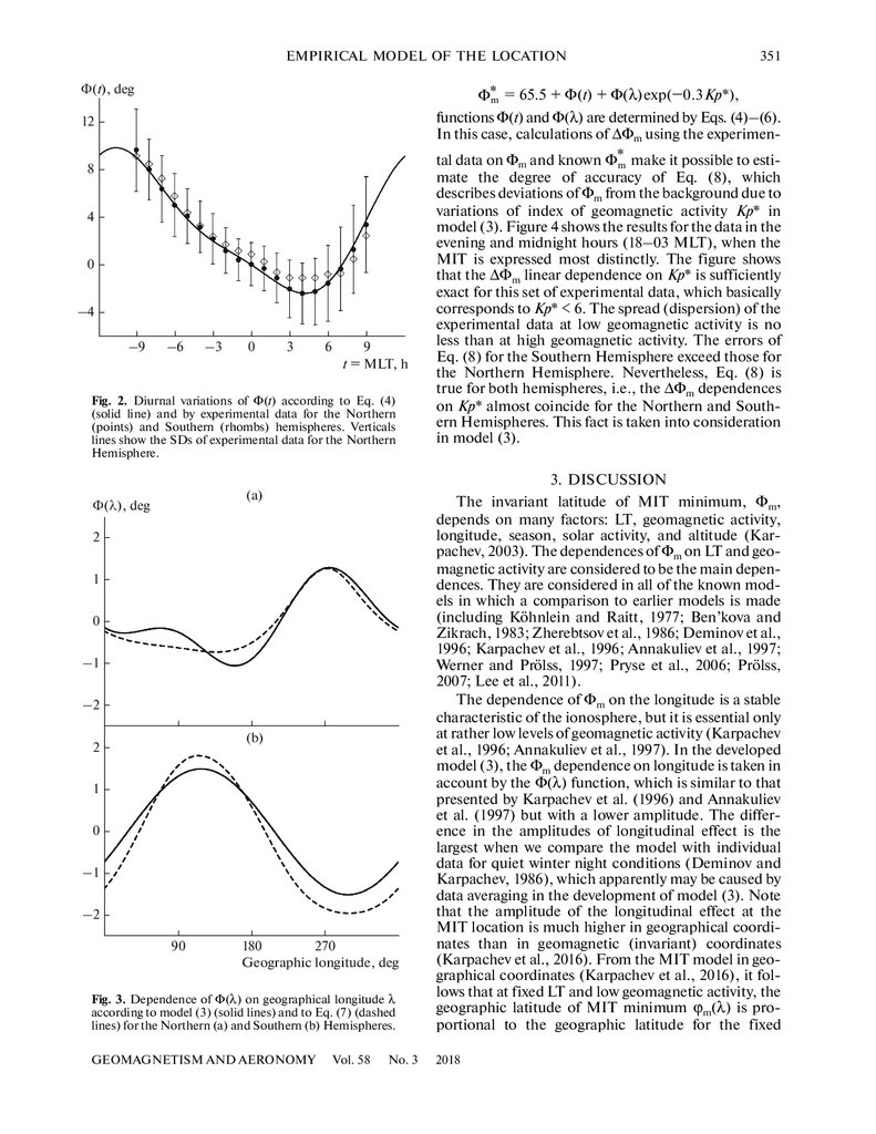
Fig. 2. Diurnal variations of Φ(t) according to Eq. (4)
(solid line) and by experimental data for the Northern
(points) and Southern (rhombs) hemispheres. Verticals
lines show the SDs of experimental data for the Northern
Hemisphere.
351
Φ*m = 65.5 + Φ(t) + Φ(λ)exp(−0.3Kp*),
functions Φ(t) and Φ(λ) are determined by Eqs. (4)–(6).
In this case, calculations of ΔΦm using the experimental data on Φm and known Φ*m make it possible to estimate the degree of accuracy of Eq. (8), which
describes deviations of Φm from the background due to
variations of index of geomagnetic activity Kp* in
model (3). Figure 4 shows the results for the data in the
evening and midnight hours (18–03 MLT), when the
MIT is expressed most distinctly. The figure shows
that the ΔΦm linear dependence on Kp* is sufficiently
exact for this set of experimental data, which basically
corresponds to Kp* < 6. The spread (dispersion) of the
experimental data at low geomagnetic activity is no
less than at high geomagnetic activity. The errors of
Eq. (8) for the Southern Hemisphere exceed those for
the Northern Hemisphere. Nevertheless, Eq. (8) is
true for both hemispheres, i.e., the ΔΦm dependences
on Kp* almost coincide for the Northern and Southern Hemispheres. This fact is taken into consideration
in model (3).
Fig. 3. Dependence of Φ(λ) on geographical longitude λ
according to model (3) (solid lines) and to Eq. (7) (dashed
lines) for the Northern (a) and Southern (b) Hemispheres.
3. DISCUSSION
The invariant latitude of MIT minimum, Φm,
depends on many factors: LT, geomagnetic activity,
longitude, season, solar activity, and altitude (Karpachev, 2003). The dependences of Φm on LT and geomagnetic activity are considered to be the main dependences. They are considered in all of the known models in which a comparison to earlier models is made
(including Köhnlein and Raitt, 1977; Ben’kova and
Zikrach, 1983; Zherebtsov et al., 1986; Deminov et al.,
1996; Karpachev et al., 1996; Annakuliev et al., 1997;
Werner and Prölss, 1997; Pryse et al., 2006; Prölss,
2007; Lee et al., 2011).
The dependence of Φm on the longitude is a stable
characteristic of the ionosphere, but it is essential only
at rather low levels of geomagnetic activity (Karpachev
et al., 1996; Annakuliev et al., 1997). In the developed
model (3), the Φm dependence on longitude is taken in
account by the Φ(λ) function, which is similar to that
presented by Karpachev et al. (1996) and Annakuliev
et al. (1997) but with a lower amplitude. The difference in the amplitudes of longitudinal effect is the
largest when we compare the model with individual
data for quiet winter night conditions (Deminov and
Karpachev, 1986), which apparently may be caused by
data averaging in the development of model (3). Note
that the amplitude of the longitudinal effect at the
MIT location is much higher in geographical coordinates than in geomagnetic (invariant) coordinates
(Karpachev et al., 2016). From the MIT model in geographical coordinates (Karpachev et al., 2016), it follows that at fixed LT and low geomagnetic activity, the
geographic latitude of MIT minimum ϕm(λ) is proportional to the geographic latitude for the fixed
GEOMAGNETISM AND AERONOMY
2018
(a)
Φ(λ), deg
2
1
0
–1
–2
(b)
2
1
0
–1
–2
90
180
270
Geographic longitude, deg
Vol. 58
No. 3
5.
352DEMINOV, SHUBIN
invariant latitude ϕ(Φ0 = const, λ). Taking Eq. (7) into
account, we obtain the following ratio
(a)
ΔΦm, deg
Φm(λ) ∼ –0.1(|ϕm(λ)| – Φ0),
where Φ0 is the mean value of the invariant latitude of
MIT minimum for the given LT at low geomagnetic
activity, which is approximately equal to the mean
(over all longitudes) value of the module of geographic
latitude of MIT minimum for these conditions. We see
from this ratio that the amplitude of the longitudinal
effect in the MIT position in geographical coordinates
is on average much higher than that in geomagnetic
coordinates. The longitudinal dependences of Φm and
ϕm are of opposite phases. This means that the longitudinal effect in the MIT location in geomagnetic
coordinates “is intended” to reduce the effect amplitude in geographical coordinates by about 5–10%.
This estimation is obtained for Kp* ~ 2 with consideration of Eq. (7) and the dependence of the amplitude
of the longitudinal effect in the MIT location on Kp*
(Eq. (3)), i.e., Φm(λ) = Φ(λ)exp(−0.3Kp*).
The dependence of the MIT minimum localization
on the solar activity is described in the MIT model in
geographical coordinates developed for winter conditions at low geomagnetic activity (Kp = 2), low
(F10.7 = 70) and high (F10.7 = 200) solar activity
(Karpachev et al., 2016). According to this model, the
MIT minimum is located at lower latitudes (i.e. equatorward) during high solar activity than at low activity.
For the interval of 18–06 SLT, this difference is maximal in the morning hours at longitudes 270°–300° E,
where it reaches 3° for the Northern Hemisphere and
5° for the Southern Hemisphere (Karpachev et al.,
2016). The dependence of the MIT localization on the
season appears to be weak, while there is a clear
dependence of the probability of MIT observation on
the season (Karpachev and Afonin, 1998). In the
developed model (3), there are no dependences of
MIT localization on the solar activity or the season,
since they have not been differentiated confidently on
the background of Φm dependence on LT and geomagnetic activity. Nevertheless, rather large errors of
model (3) for the Southern Hemisphere (see Fig. 4)
and during morning hours for the Northern Hemisphere (see Fig. 2) show that not all factors have been
considered in this model, which would influence the
MIT minimum localization.
We carried out a more detailed comparison of the
developed model (3) with the known Φm models presented in the literature (Köhnlein and Raitt, 1977;
Ben’kova and Zikrach, 1983; Zherebtsov et al., 1986;
Karpachev et al., 1996; Annakuliev et al., 1997; Werner and Prölss, 1997; Pryse et al., 2006; Prölss, 2007).
Different indices of geomagnetic activity are used in
these models. For a qualitative comparison of the
models, the indices are reduced to the Kp index by the
relations
Kp* = Kp,
AE6 = −4 + 122Kp,
0
–10
–20
σ = 1.97
(b)
0
–10
–20
σ = 2.83
2
4
6
Kp*
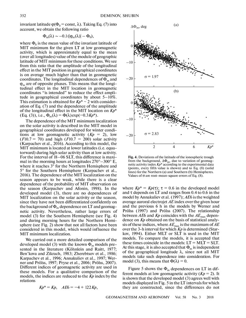
Fig. 4. Deviations of the latitude of the ionospheric trough
from the background, ΔΦm, due to variation of geomagnetic activity index Kp* according to the experimental data
(points, every fifth value is shown) and to Eq. (8) (solid
lines) for the Northern (a) and Southern (b) Hemispheres.
Values of σ are root-mean-square errors of Eq. (8).
where Kp* = Kp(τ); τ = 0.6 in the developed model
and τ depends on LT and ranges from 0.4 to 0.6 in the
model by Annakuliev et al. (1997); AE6 is the weighted
average auroral electrojet AE index over the given hour
and the previous 6 h in the models by Werner and
Prölss (1997) and Prölss (2007). The relationship
between AE6 and Kp coincides with the AEmax dependence on Kp obtained on the basis of statistical analysis of these indices, where AEmax is the maximum of AE
over the 3-h interval for which Kp is determined (Starkov, 1994). Either MLT or SLT is used in the MIT
models. To compare the models, it is accepted that
these times coincide in the models: LT = MLT = SLT.
At this stage, it is also accepted that Φm is independent
of the geographical longitude λ, since not all MIT
models take such dependence into consideration. For
model (3), this means that Φ(λ) = 0.
Figure 5 shows the Φm dependences on LT in different models at low geomagnetic activity (Kp = 2). It
is shown that the developed model (3) agrees well with
models displayed in Fig. 5 in the LT intervals for which
they are constructed, since the differences do not
GEOMAGNETISM AND AERONOMY
Vol. 58
No. 3
2018
6.
EMPIRICAL MODEL OF THE LOCATIONΦm, deg
70
68
66
1
64
3
62
2
60
4
58
–9
–6
–3
0
6
3
9 LT, h
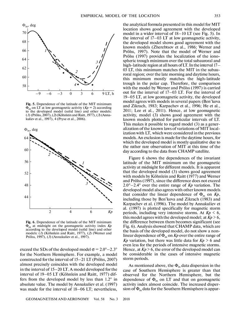
Fig. 5. Dependence of the latitude of the MIT minimum
Φm on LT at low geomagnetic activity (Kp = 2) according
to the developed model (solid line) and other models:
(1) (Prölss, 2007), (2) (Köhnlein and Raitt, 1977), (3) (Annakuliev et al., 1997), 4 (Pryse et al., 2006).
Φm, deg
64
60
2
56
1
52
3
48
44
2
4
Kp
6
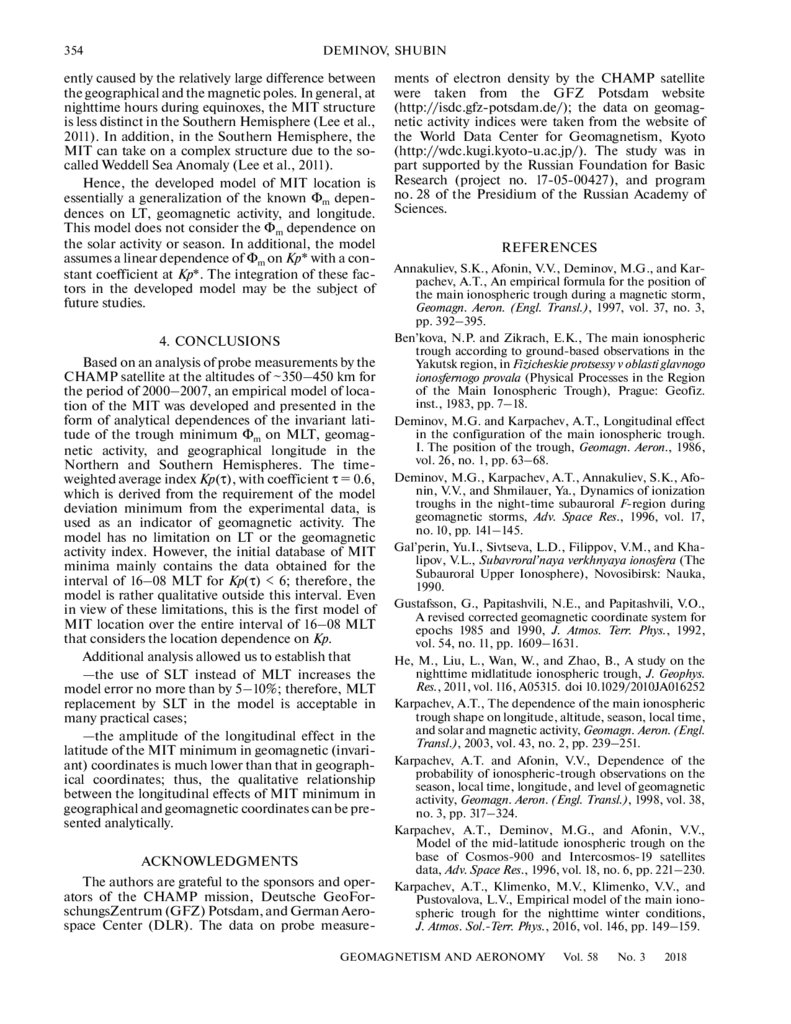
Fig. 6. Dependence of the latitude of the MIT minimum
Φm at midnight on the geomagnetic activity index Kp
according to the developed model (solid line) and other
models: (1) (Köhnlein and Raitt, 1977), (2) (Werner and
Prölss, 1997), (3) (Annakuliev et al., 1997).
exceed the SDs of the developed model σ = 2.0°–2.3°
for the Northern Hemisphere. For example, a model
constructed for the interval of 15–21 LT (Prölss, 2007)
almost precisely coincides with the developed model
in the interval of 15–20 LT. A model developed for the
interval of 19–05 LT (Köhnlein and Raitt, 1977) differs from the developed model by less than 1.2° in
absolute value. The model by Annakuliev et al. (1997)
was made for the interval of 18–06 LT; nevertheless,
GEOMAGNETISM AND AERONOMY
Vol. 58
No. 3
353
the analytical formula presented in this model for MIT
location shows good agreement with the developed
model in a wider interval of 18–10 LT (see Fig. 5). In
the interval of 17–03 LT at low geomagnetic activity,
the developed model shows good agreement with the
known models (Zherebtsov et al., 1986; Werner and
Prölss, 1997). Note that the model of Werner and
Prölss (1997) provides the localization of the ionospheric trough minimum over the total subauroral and
high-latitude region at all hours of LT. In the interval 17–
03 LT, this minimum matches the MIT in the subauroral region; over the late morning and daytime hours,
this minimum mostly matches the high-latitude
trough in the polar cap. Therefore, the comparison
with the model by Werner and Prölss (1997) is carried
out for the interval of 17–03 LT. For the interval of
19–05 LT, at low geomagnetic activity, the developed
model agrees with models in several papers (Ben’kova
and Zikrach, 1983; Karpachev et al., 1996; He et al.,
2011; Lee et al., 2011). Hence, at low geomagnetic
activity, model (3) shows good agreement with the
known models plotted for particular intervals of LT.
This makes it possible to regard model (3) as a generalization of the known laws of variations of MIT localization with LT, which were considered in the previous
models. An exclusion is made for the daytime hours, for
which the developed model is mostly qualitative due to
the rather rare observation of MIT at this time of the
day according to the data from CHAMP satellite.
Figure 6 shows the dependences of the invariant
latitude of the MIT minimum on the geomagnetic
activity at midnight for different models. It is apparent
that the developed model (3) shows good agreement
with models by Köhnlein and Raitt (1977) and Werner
and Prölss (1997), since the difference does not exceed
2.0°–2.4° over the entire range of Kp variation. The
developed model also agrees with other known models
that consider the linear dependence of Φm on Kp,
including those by Ben’kova and Zikrach (1983) and
Karpachev et al. (1996). The model by Annakuliev et
al. (1997) is plotted specifically for magnetic storm
periods, including very intensive storms. At Kp < 6,
this model agrees with the developed model; at Kp > 6,
the difference between them becomes significant (see
Fig. 6). Analysis showed that CHAMP data, which are
the basis of the developed model, do not show a nonlinear dependence of Φm on Kp over the entire range of
Kp variation, but there was little data for Kp > 6 and
even less for the periods of intensive magnetic storms.
Hence, at Kp > 6, the error of the developed model can
be considerable in the cases of intensive magnetic
storm periods.
As mentioned above, the Φm data dispersion in the
case of Southern Hemisphere is greater than that
observed for the Northern Hemisphere, but the
dependence of Φm on LT and that on geomagnetic
activity index almost coincide. The increased dispersion of Φm data for the Southern Hemisphere is appar2018
7.
354DEMINOV, SHUBIN
ently caused by the relatively large difference between
the geographical and the magnetic poles. In general, at
nighttime hours during equinoxes, the MIT structure
is less distinct in the Southern Hemisphere (Lee et al.,
2011). In addition, in the Southern Hemisphere, the
MIT can take on a complex structure due to the socalled Weddell Sea Anomaly (Lee et al., 2011).
Hence, the developed model of MIT location is
essentially a generalization of the known Φm dependences on LT, geomagnetic activity, and longitude.
This model does not consider the Φm dependence on
the solar activity or season. In additional, the model
assumes a linear dependence of Φm on Kp* with a constant coefficient at Kp*. The integration of these factors in the developed model may be the subject of
future studies.
4. CONCLUSIONS
Based on an analysis of probe measurements by the
CHAMP satellite at the altitudes of ~350–450 km for
the period of 2000–2007, an empirical model of location of the MIT was developed and presented in the
form of analytical dependences of the invariant latitude of the trough minimum Φm on MLT, geomagnetic activity, and geographical longitude in the
Northern and Southern Hemispheres. The timeweighted average index Kp(τ), with coefficient τ = 0.6,
which is derived from the requirement of the model
deviation minimum from the experimental data, is
used as an indicator of geomagnetic activity. The
model has no limitation on LT or the geomagnetic
activity index. However, the initial database of MIT
minima mainly contains the data obtained for the
interval of 16–08 MLT for Kp(τ) < 6; therefore, the
model is rather qualitative outside this interval. Even
in view of these limitations, this is the first model of
MIT location over the entire interval of 16–08 MLT
that considers the location dependence on Kp.
Additional analysis allowed us to establish that
—the use of SLT instead of MLT increases the
model error no more than by 5–10%; therefore, MLT
replacement by SLT in the model is acceptable in
many practical cases;
—the amplitude of the longitudinal effect in the
latitude of the MIT minimum in geomagnetic (invariant) coordinates is much lower than that in geographical coordinates; thus, the qualitative relationship
between the longitudinal effects of MIT minimum in
geographical and geomagnetic coordinates can be presented analytically.
ACKNOWLEDGMENTS
The authors are grateful to the sponsors and operators of the CHAMP mission, Deutsche GeoForschungsZentrum (GFZ) Potsdam, and German Aerospace Center (DLR). The data on probe measure-
ments of electron density by the CHAMP satellite
were taken from the GFZ Potsdam website
(http://isdc.gfz-potsdam.de/); the data on geomagnetic activity indices were taken from the website of
the World Data Center for Geomagnetism, Kyoto
(http://wdc.kugi.kyoto-u.ac.jp/). The study was in
part supported by the Russian Foundation for Basic
Research (project no. 17-05-00427), and program
no. 28 of the Presidium of the Russian Academy of
Sciences.
REFERENCES
Annakuliev, S.K., Afonin, V.V., Deminov, M.G., and Karpachev, A.T., An empirical formula for the position of
the main ionospheric trough during a magnetic storm,
Geomagn. Aeron. (Engl. Transl.), 1997, vol. 37, no. 3,
pp. 392–395.
Ben’kova, N.P. and Zikrach, E.K., The main ionospheric
trough according to ground-based observations in the
Yakutsk region, in Fizicheskie protsessy v oblasti glavnogo
ionosfernogo provala (Physical Processes in the Region
of the Main Ionospheric Trough), Prague: Geofiz.
inst., 1983, pp. 7–18.
Deminov, M.G. and Karpachev, A.T., Longitudinal effect
in the configuration of the main ionospheric trough.
I. The position of the trough, Geomagn. Aeron., 1986,
vol. 26, no. 1, pp. 63–68.
Deminov, M.G., Karpachev, A.T., Annakuliev, S.K., Afonin, V.V., and Shmilauer, Ya., Dynamics of ionization
troughs in the night-time subauroral F-region during
geomagnetic storms, Adv. Space Res., 1996, vol. 17,
no. 10, pp. 141–145.
Gal’perin, Yu.I., Sivtseva, L.D., Filippov, V.M., and Khalipov, V.L., Subavroral’naya verkhnyaya ionosfera (The
Subauroral Upper Ionosphere), Novosibirsk: Nauka,
1990.
Gustafsson, G., Papitashvili, N.E., and Papitashvili, V.O.,
A revised corrected geomagnetic coordinate system for
epochs 1985 and 1990, J. Atmos. Terr. Phys., 1992,
vol. 54, no. 11, pp. 1609–1631.
He, M., Liu, L., Wan, W., and Zhao, B., A study on the
nighttime midlatitude ionospheric trough, J. Geophys.
Res., 2011, vol. 116, A05315. doi 10.1029/2010JA016252
Karpachev, A.T., The dependence of the main ionospheric
trough shape on longitude, altitude, season, local time,
and solar and magnetic activity, Geomagn. Aeron. (Engl.
Transl.), 2003, vol. 43, no. 2, pp. 239–251.
Karpachev, A.T. and Afonin, V.V., Dependence of the
probability of ionospheric-trough observations on the
season, local time, longitude, and level of geomagnetic
activity, Geomagn. Aeron. (Engl. Transl.), 1998, vol. 38,
no. 3, pp. 317–324.
Karpachev, A.T., Deminov, M.G., and Afonin, V.V.,
Model of the mid-latitude ionospheric trough on the
base of Cosmos-900 and Intercosmos-19 satellites
data, Adv. Space Res., 1996, vol. 18, no. 6, pp. 221–230.
Karpachev, A.T., Klimenko, M.V., Klimenko, V.V., and
Pustovalova, L.V., Empirical model of the main ionospheric trough for the nighttime winter conditions,
J. Atmos. Sol.-Terr. Phys., 2016, vol. 146, pp. 149–159.
GEOMAGNETISM AND AERONOMY
Vol. 58
No. 3
2018
8.
EMPIRICAL MODEL OF THE LOCATIONKöhnlein, W. and Raitt, W.I., Position of mid-latitude
trough in the topside ionosphere as deduced from
ESRO-4 observations, Planet. Space Sci., 1977, vol. 25,
no. 6, pp. 600–602.
Lee, I.T., Wang, W., Liu, J.Y., Chen, C.Y., and Lin, C.H.,
The ionospheric midlatitude trough observed by
FORMOSAT-3/COSMIC during solar minimum,
J. Geophys. Res., 2011, vol. 116, A06311.
doi
10.1029/2010JA015544
Moffett, R. and Quegan, S., The mid-latitude trough in the
electron concentration of the ionospheric F-layer: A
review of observations and modelling, J. Atmos. Terr.
Phys., 1983, vol. 45, no. 5, pp. 315–343.
Prölss, G.W., The equatorward wall of the subauroral
trough in the afternoon/evening sector, Ann. Geophys.,
2007, vol. 25, no. 3, pp. 645–659.
Pryse, S.E., Kersley, L., Malan, D., and Bishop, G.J.,
Parameterization of the main ionospheric trough in the
European sector, Radio Sci., 2006, vol. 41, RS5S14.
doi 10.1029/2005RS003364
Rodger, A., Moffett, R., and Quegan, S., The role of ion
drift in the formation of ionisation troughs in the midand high-latitude ionosphere: A review, J. Atmos. Terr.
Phys., 1992, vol. 54, no. 1, pp. 1–30.
GEOMAGNETISM AND AERONOMY
Vol. 58
No. 3
355
Starkov, G.V., Statistical dependences between magnetic
activity indices, Geomagn. Aeron., 1994, vol. 34, no. 1,
pp. 129–131.
Themens, D.R., Jayachandran, P.T., Galkin, I., and Hall, C.,
The empirical Canadian high Arctic ionospheric model
(E-CHAIM): NmF2 and hmF2, J. Geophys. Res.: Space
Phys., 2017, vol. 122, no. 8. doi 10.1002/2017JA024398
Werner, S. and Prölss, G.W., The position of the ionospheric trough as a function of local time and magnetic
activity, Adv. Space Res., 1997, vol. 20, no. 9, pp. 1717–
1722.
Wrenn, G.L., Time-weighted accumulations ap(τ) and
Kp(τ), J. Geophys. Res., 1987, vol. 92, pp. 10125–10129.
Yang, N., Le, H., and Liu, L., Statistical analysis of the
mid-latitude trough position during different categories
of magnetic storms and different storm intensities,
Earth Planets Space, 2016, vol. 68. doi 10.1186/s40623016-0554-6
Zherebtsov, G.A., Pirog, O.M., and Razuvaev, O.I., The
structure and dynamics of the high-latitude ionosphere, in Issled. po geomagnetizmu, aeronomii i fizike
Solntsa (Studies on Geomagnetism, Aeronomy, and
Solar Physics), Moscow: Nauka, 1986, vol. 68, pp. 165–
177.
Translated by N. Semenova
2018